
Access CCMP data on Pangeo
This tutorial shows how to access the CCMP wind speed data, makes a few plots of the data, and then compares it to a buoy wind speed.
CCMP Winds in a cloud-optimized-format for Pangeo
The Cross-Calibrated Multi-Platform (CCMP) Ocean Surface Wind Vector Analyses is part of the NASA Making Earth System Data Records for Use in Research Environments (MEaSUREs) Program. MEaSUREs, develops consistent global- and continental-scale Earth System Data Records by supporting projects that produce data using proven algorithms and input. If you use this data, please give credit. For more information, please review the documentation. Please note that this data is not recommended for trend calculations.
Data is NRT from 4/1/2019 - 10/4/2020. The 6-hourly VAM analyses are centered at 0,6,12 and 18z
Accessing cloud satellite data
CCMP zarr conversion funding: Interagency Implementation and Advanced Concepts Team IMPACT for the Earth Science Data Systems (ESDS) program and AWS Public Dataset Program
Credit:
Chelle Gentemann, Farallon Institute, Twitter - creation of Zarr data store and tutorial
Charles Blackmon Luca, LDEO - help with moving to Pangeo storage and intake update
Willi Rath, GEOMAR, Twitter - motivated CG to move data to Pangeo!
Tom Augspurger, Microsoft,Twitter - help updating the data.
Zarr data format
Data proximate computing
To run this notebook
Code is in the cells that have In [ ]: to the left of the cell and have a colored background
To run the code: - option 1) click anywhere in the cell, then hold shift down and press Enter - option 2) click on the Run button at the top of the page in the dashboard
Remember: - to insert a new cell below press Esc then b - to delete a cell press Esc then dd
First start by importing libraries
[1]:
#libs for reading data
import xarray as xr
import intake
import numpy as np
import matplotlib.pyplot as plt
from matplotlib.dates import DateFormatter
import cartopy.crs as ccrs

#lib for dask gateway
from dask_gateway import Gateway
from dask.distributed import Client
from dask import delayed
/srv/conda/envs/notebook/lib/python3.8/site-packages/dask_gateway/client.py:21: FutureWarning: format_bytes is deprecated and will be removed in a future release. Please use dask.utils.format_bytes instead.
  from distributed.utils import LoopRunner, format_bytes
Start a cluster, a group of computers that will work together.
(A cluster is the key to big data analysis on on Cloud.)
This will set up a dask kubernetes cluster for your analysis and give you a path that you can paste into the top of the Dask dashboard to visualize parts of your cluster.
You don’t need to paste the link below into the Dask dashboard for this to work, but it will help you visualize progress.
Try 20 workers to start (during the tutorial) but you can increase to speed things up later
[2]:
gateway = Gateway()
cluster = gateway.new_cluster()
cluster.adapt(minimum=1, maximum=75)
client = Client(cluster)
cluster
** ☝️ Don’t forget to click the link above or copy it to the Dask dashboard (orange icon) on the left to view the scheduler dashboard! **
Initialize Dataset
Here we load the dataset from the zarr store. Note that this very large dataset (273 GB) initializes nearly instantly, and we can see the full list of variables and coordinates.
Examine Metadata
For those unfamiliar with this dataset, the variable metadata is very helpful for understanding what the variables actually represent Printing the dataset will show you the dimensions, coordinates, and data variables with clickable icons at the end that show more metadata and size.
[3]:
%%time
cat_pangeo = intake.open_catalog("https://raw.githubusercontent.com/pangeo-data/pangeo-datastore/master/intake-catalogs/master.yaml")

ds_ccmp = cat_pangeo.atmosphere.nasa_ccmp_wind_vectors.to_dask()

#calculate wind speed and add attributes to new variable
ds_ccmp['wspd'] = np.sqrt(ds_ccmp.uwnd**2 + ds_ccmp.vwnd**2)
ds_ccmp.wspd.attrs=ds_ccmp.uwnd.attrs
ds_ccmp.wspd.attrs['long_name']='wind speed at 10 meters'

ds_ccmp
CPU times: user 650 ms, sys: 92.5 ms, total: 743 ms
Wall time: 1.42 s
[3]:
<xarray.Dataset>
Dimensions:    (latitude: 628, longitude: 1440, time: 48392)
Coordinates:
  * latitude   (latitude) float32 -78.38 -78.12 -77.88 ... 77.88 78.12 78.38
  * longitude  (longitude) float32 0.125 0.375 0.625 0.875 ... 359.4 359.6 359.9
  * time       (time) datetime64[ns] 1987-07-10 ... 2020-10-04T18:00:00
Data variables:
    nobs       (time, latitude, longitude) float32 dask.array<chunksize=(2000, 157, 180), meta=np.ndarray>
    uwnd       (time, latitude, longitude) float32 dask.array<chunksize=(2000, 157, 180), meta=np.ndarray>
    vwnd       (time, latitude, longitude) float32 dask.array<chunksize=(2000, 157, 180), meta=np.ndarray>
    wspd       (time, latitude, longitude) float32 dask.array<chunksize=(2000, 157, 180), meta=np.ndarray>
Attributes: (12/36)
    Conventions:                CF-1.6
    base_date:                  Y2020 M08 D06
    comment:                    none
    contact:                    Remote Sensing Systems, support@remss.com
    contributor_name:           Carl Mears, Joel Scott, Frank Wentz, Ross Hof...
    contributor_role:           Co-Investigator, Software Engineer, Project L...
    ...                         ...
    publisher_email:            support@remss.com
    publisher_name:             Remote Sensing Systems
    publisher_url:              http://www.remss.com/
    references:                 Hoffman et al., Journal of Atmospheric and Oc...
    summary:                    CCMP_RT V2.1 has been created using the same ...
title: RSS CCMP_RT V2.1 derived surface winds (Level...- latitude: 628
- longitude: 1440
- time: 48392
- latitude(latitude)float32-78.38 -78.12 ... 78.12 78.38
- _CoordinateAxisType :
- Lat
- _Fillvalue :
- -9999.0
- axis :
- Y
- coordinate_defines :
- center
- long_name :
- Latitude in degrees north
- standard_name :
- latitude
- units :
- degrees_north
- valid_max :
- 78.375
- valid_min :
- -78.375
array([-78.375, -78.125, -77.875, ..., 77.875, 78.125, 78.375], dtype=float32) - longitude(longitude)float320.125 0.375 0.625 ... 359.6 359.9
- _CoordinateAxisType :
- Lon
- _Fillvalue :
- -9999.0
- axis :
- X
- coordinate_defines :
- center
- long_name :
- Longitude in degrees east
- standard_name :
- longitude
- units :
- degrees_east
- valid_max :
- 359.875
- valid_min :
- 0.125
array([1.25000e-01, 3.75000e-01, 6.25000e-01, ..., 3.59375e+02, 3.59625e+02, 3.59875e+02], dtype=float32) - time(time)datetime64[ns]1987-07-10 ... 2020-10-04T18:00:00
- _CoordinateAxisType :
- Time
- _Fillvalue :
- -9999.0
- axis :
- T
- long_name :
- Time of analysis
- standard_name :
- time
array(['1987-07-10T00:00:00.000000000', '1987-07-10T06:00:00.000000000',
       '1987-07-10T12:00:00.000000000', ..., '2020-10-04T06:00:00.000000000',
       '2020-10-04T12:00:00.000000000', '2020-10-04T18:00:00.000000000'],
      dtype='datetime64[ns]')
- nobs(time, latitude, longitude)float32dask.array<chunksize=(2000, 157, 180), meta=np.ndarray>
- _Fillvalue :
- -9999.0
- ancillary_variables :
- uwnd vwnd
- long_name :
- number of observations used to derive wind vector components
- standard_name :
- number_of_observations
- units :
- count
- valid_max :
- 2.0
- valid_min :
- 0.0
Array Chunk Bytes 163.03 GiB 215.61 MiB Shape (48392, 628, 1440) (2000, 157, 180) Count 801 Tasks 800 Chunks Type float32 numpy.ndarray - uwnd(time, latitude, longitude)float32dask.array<chunksize=(2000, 157, 180), meta=np.ndarray>
- _Fillvalue :
- -9999.0
- height :
- 10 meters above sea-level
- long_name :
- u-wind vector component at 10 meters
- standard_name :
- eastward_wind
- units :
- m s-1
- valid_max :
- 20.291385650634766
- valid_min :
- -21.261892318725586
Array Chunk Bytes 163.03 GiB 215.61 MiB Shape (48392, 628, 1440) (2000, 157, 180) Count 801 Tasks 800 Chunks Type float32 numpy.ndarray - vwnd(time, latitude, longitude)float32dask.array<chunksize=(2000, 157, 180), meta=np.ndarray>
- _Fillvalue :
- -9999.0
- height :
- 10 meters above sea-level
- long_name :
- v-wind vector component at 10 meters
- standard_name :
- northward_wind
- units :
- m s-1
- valid_max :
- 22.860544204711914
- valid_min :
- -18.280412673950195
Array Chunk Bytes 163.03 GiB 215.61 MiB Shape (48392, 628, 1440) (2000, 157, 180) Count 801 Tasks 800 Chunks Type float32 numpy.ndarray - wspd(time, latitude, longitude)float32dask.array<chunksize=(2000, 157, 180), meta=np.ndarray>
- _Fillvalue :
- -9999.0
- height :
- 10 meters above sea-level
- long_name :
- wind speed at 10 meters
- standard_name :
- eastward_wind
- units :
- m s-1
- valid_max :
- 20.291385650634766
- valid_min :
- -21.261892318725586
Array Chunk Bytes 163.03 GiB 215.61 MiB Shape (48392, 628, 1440) (2000, 157, 180) Count 4802 Tasks 800 Chunks Type float32 numpy.ndarray
- Conventions :
- CF-1.6
- base_date :
- Y2020 M08 D06
- comment :
- none
- contact :
- Remote Sensing Systems, support@remss.com
- contributor_name :
- Carl Mears, Joel Scott, Frank Wentz, Ross Hoffman, Mark Leidner, Robert Atlas, Joe Ardizzone
- contributor_role :
- Co-Investigator, Software Engineer, Project Lead, Co-Investigator, Software Engineer, Principal Investigator, Software Engineer
- creator_email :
- support@remss.com
- creator_name :
- Remote Sensing Systems
- creator_url :
- http://www.remss.com/
- data_structure :
- grid
- date_created :
- 20200820T130255Z
- description :
- RSS VAM 6-hour analyses starting from the NCEP GFS wind analyses
- geospatial_lat_max :
- 78.375 degrees
- geospatial_lat_min :
- -78.375 degrees
- geospatial_lat_resolution :
- 0.25 degrees
- geospatial_lat_units :
- degrees_north
- geospatial_lon_max :
- 359.875 degrees
- geospatial_lon_min :
- 0.125 degrees
- geospatial_lon_resolution :
- 0.25 degrees
- geospatial_lon_units :
- degrees_east
- history :
- 20200820T130255ZZ - netCDF generated from original data using IDL 8.5 by RSS using files: CCMP_RT_Wind_Analysis_20200806_V02.0_L3.0_RSS.nc
- institute_id :
- RSS
- institution :
- Remote Sensing Systems (RSS)
- keywords :
- surface winds, ocean winds, wind speed/wind direction, MEaSUREs, 10km - < 50km or approximately 0.09 degree - < 0.5 degree
- keywords_vocabulary :
- GCMD Science Keywords
- license :
- available for public use with proper citation
- netcdf_version_id :
- 4.2
- processing_level :
- L3.0
- product_version :
- v2.1
- project :
- RSS Cross-Calibrated Multi-Platform Ocean Surface Wind Project
- publisher_email :
- support@remss.com
- publisher_name :
- Remote Sensing Systems
- publisher_url :
- http://www.remss.com/
- references :
- Hoffman et al., Journal of Atmospheric and Oceanic Technology, 2013; Atlas et al., BAMS, 2011; Atlas et al., BAMS, 1996
- summary :
- CCMP_RT V2.1 has been created using the same VAM as CCMP V2.0 Input data have changed and now include all V7 radiometer data from RSS, V8.1 GMI data from RSS, scatterometer data from RSS (V4 QuikSCAT and V1.2 ASCAT), quality checked moored buoy data from NDBC, PMEL, and ISDM, and NCEP GFS 0.25 degree data for the background field.
- title :
- RSS CCMP_RT V2.1 derived surface winds (Level 3.0)
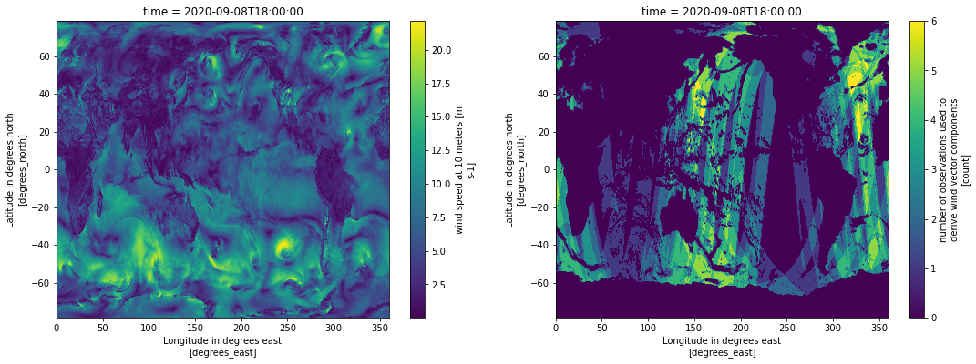
Plot a global image of the data on 7/4/2020 (randomly chosen day)
xarray makes plotting the data very easy. A nice overview of plotting with xarray is here. Details on .plot
Below we are plotting the variable wspd (wind speed) and nobs (number of observations) to show how there is data over the ocean but none over land. CCMP data includes 25 km ERA5 data over land.
[4]:
%%time

day = ds_ccmp.sel(time='2020-09-08T18')

fig, ax = plt.subplots(1,2, figsize=(18,6))

day.wspd.plot(ax=ax[0])

day.nobs.plot(ax=ax[1])
CPU times: user 767 ms, sys: 190 ms, total: 956 ms
Wall time: 3min
[4]:
<matplotlib.collections.QuadMesh at 0x7f32c613eb80>
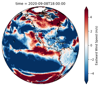
[5]:
import cartopy
import cartopy.crs as ccrs
ortho = ccrs.Orthographic(-110, 20)           # define target coordinate frame
geo = ccrs.PlateCarree()                     # define origin coordinate frame

plt.figure(figsize=(7,5))                    #set the figure size
ax = plt.subplot(1, 1, 1, projection=ortho)  #create the axis for plotting
q = day.uwnd.plot(ax=ax,
                            transform = geo,
                            cmap='RdBu_r', #'cmo.thermal',
                            vmin=-5,
                            vmax=5,cbar_kwargs={'label':'Eastward Wind Speed (m/s)'}) # plot a colormap in transformed coordinates cmap='OrRd',
global_extent = ax.get_extent(crs=ccrs.PlateCarree())
#ax.add_feature(cartopy.feature.LAND,color='gray')
ax.add_feature(cartopy.feature.COASTLINE)

#plt.savefig('./../../figures/ccmp_wind_example.png')
[5]:
<cartopy.mpl.feature_artist.FeatureArtist at 0x7f32c61f4250>
/srv/conda/envs/notebook/lib/python3.8/site-packages/cartopy/io/__init__.py:241: DownloadWarning: Downloading: https://naciscdn.org/naturalearth/110m/physical/ne_110m_coastline.zip
  warnings.warn('Downloading: {}'.format(url), DownloadWarning)
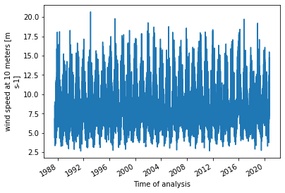
Plot a timeseries of the average wind speed over a region
use .sel and slice to select a region of data
use .mean to calculate the spatial mean
use .plot to plot a timeseries of the mean wind speed
[6]:
%%time

subset = ds_ccmp.sel(latitude=slice(30,50),longitude=slice(200,210))

ts = subset.mean({'latitude','longitude'},keep_attrs=True)

ts.wspd.plot()
CPU times: user 203 ms, sys: 22.5 ms, total: 225 ms
Wall time: 48.7 s
[6]:
[<matplotlib.lines.Line2D at 0x7f32c60e8940>]
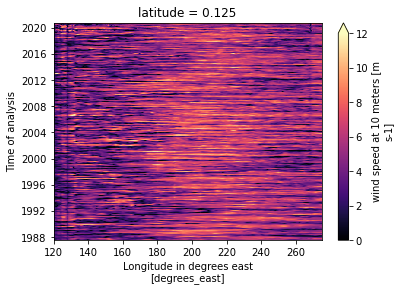
Make a Hovmoller diagram
Hovmoller diagrams are common plots in oceanography and meteorology to look at propogation of waves. They often have latitude or longitude along the x-axis and time along the y-axis so you can look at how things propogate in time.
[7]:
%%time

ds_ccmp.sel(latitude=0.125,longitude=slice(120,275)).wspd.plot(vmin=0,vmax=12,cmap='magma')
distributed.client - WARNING - Couldn't gather 2 keys, rescheduling {"('getitem-7680cdf45141faec63b553a96087af16', 1, 3)": (), "('getitem-7680cdf45141faec63b553a96087af16', 4, 3)": ()}
CPU times: user 3.12 s, sys: 533 ms, total: 3.65 s
Wall time: 2min 7s
[7]:
<matplotlib.collections.QuadMesh at 0x7f32c5fe6d60>
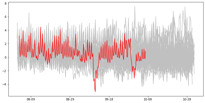
In Feb 2020 a GRL paper came out connecting 3 closely occuring Typhoons near Korea to the California wildfires
“Strong winds that accentuated a fire outbreak in the western United States in early September of 2020 resulted from an atmospheric wave train that spanned the Pacific Ocean. Days before the atmospheric waves developed in the United States, three western Pacific tropical cyclones (typhoons) underwent an extratropical transition over Korea within an unprecedentedly short span of 12 days.”
Using ERA5 winds, Figure 1 showed zonal winds averaged over a box located over NCal/Oregon. On 9/8 and again on 9/24 the zonal winds were strongly negative (Diablo winds) and both events were associated with major fires.
Below, let’s do the same figure with CCMP winds - Note that CCMP winds end 10/4/2020, so the data will end at that point.
First create a timeseries of the ‘uwnd’ or east-west wind vector for the same region used in the paper above.
Next plot all the data in grey and then add 2020 data in red.
[8]:
ts = ds_ccmp.uwnd.sel(longitude=slice(236,239),latitude=slice(41,46)).mean({'latitude','longitude'}).load()
[9]:
#plot the data
fig, ax = plt.subplots(figsize=(12, 6))
for lyr in range(1979,2021):
    yr = ts.sel(time=slice(str(lyr)+'-08-01',str(lyr)+'-10-29'))
    xx=yr.time.dt.dayofyear+yr.time.dt.hour/24
    ax.plot(xx,yr,color='silver')
    if lyr==2020:
        ax.plot(xx,yr,color='red')
date_form = DateFormatter("%m-%d")
ax.xaxis.set_major_formatter(date_form)
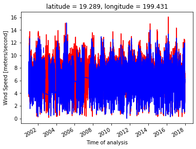
Compare the satellite wind speeds to buoy (in situ) data
Data from NDBC buoys, which measure wind speed are here and can be read via an THREDDS server. - read in NDBC buoy data - find closest CCMP data and linearly interpolate to buoy location - examine a timeseries, caluclate bias and STD
[10]:
%%time
#read in NDBC buoy data
url='https://dods.ndbc.noaa.gov/thredds/dodsC/data/cwind/51003/51003.ncml'

with xr.open_dataset(url) as ds:
    # The longitude is on a -180 to 180, CCMP is 0-360, so make sure to convert
    ds.coords['longitude'] = np.mod(ds['longitude'], 360)
ds
CPU times: user 96.2 ms, sys: 39.9 ms, total: 136 ms
Wall time: 2.27 s
[10]:
<xarray.Dataset>
Dimensions:    (latitude: 1, longitude: 1, time: 806344)
Coordinates:
  * latitude   (latitude) float32 19.29
  * longitude  (longitude) float32 199.4
  * time       (time) datetime64[ns] 2001-01-09T17:00:00 ... 2017-12-31T22:50:00
Data variables:
    wind_dir   (time, latitude, longitude) float64 ...
    wind_spd   (time, latitude, longitude) float32 ...
Attributes:
    institution:  NOAA National Data Buoy Center and Participators in Data As...
    url:          http://dods.ndbc.noaa.gov
    quality:      Automated QC checks with manual editing and comprehensive m...
    conventions:  COARDS
    station:      51003
    comment:      WESTERN  HAWAII - 205 NM SW of Honolulu, HI
location: 19.289 N 160.569 W - latitude: 1
- longitude: 1
- time: 806344
- latitude(latitude)float3219.29
- long_name :
- Latitude
- short_name :
- latitude
- standard_name :
- latitude
- units :
- degrees_north
array([19.289], dtype=float32)
- longitude(longitude)float32199.4
- long_name :
- Longitude
- short_name :
- longitude
- standard_name :
- longitude
- units :
- degrees_east
array([199.431], dtype=float32)
- time(time)datetime64[ns]2001-01-09T17:00:00 ... 2017-12-...
- long_name :
- Epoch Time
- short_name :
- time
- standard_name :
- time
array(['2001-01-09T17:00:00.000000000', '2001-01-09T17:10:00.000000000',
       '2001-01-09T17:20:00.000000000', ..., '2017-12-31T22:30:00.000000000',
       '2017-12-31T22:40:00.000000000', '2017-12-31T22:50:00.000000000'],
      dtype='datetime64[ns]')
- wind_dir(time, latitude, longitude)float64...
- long_name :
- Wind Direction
- short_name :
- wdir
- standard_name :
- wind_from_direction
- units :
- degrees_true
[806344 values with dtype=float64]
- wind_spd(time, latitude, longitude)float32...
- long_name :
- Wind Speed
- short_name :
- wspd
- standard_name :
- wind_speed
- units :
- meters/second
[806344 values with dtype=float32]
- institution :
- NOAA National Data Buoy Center and Participators in Data Assembly Center
- url :
- http://dods.ndbc.noaa.gov
- quality :
- Automated QC checks with manual editing and comprehensive monthly QC
- conventions :
- COARDS
- station :
- 51003
- comment :
- WESTERN HAWAII - 205 NM SW of Honolulu, HI
- location :
- 19.289 N 160.569 W
[11]:
%%time
#find the time period that both data exist eg. start and stop
time_start = np.max([ds.time[0].data,ds_ccmp.time[0].data])
time_stop = np.min([ds.time[-1].data,ds_ccmp.time[-1].data])

#cut off satellite data to joint period
# then linearly interpolate the data to the buoy location
ccmp_buoy = ds_ccmp.sel(time=slice(time_start,time_stop)).interp(latitude=ds.latitude,longitude=ds.longitude,method='linear')

#cut off buoy data to joint period
ds = ds.sel(time=slice(time_start,time_stop))
CPU times: user 94.1 ms, sys: 1.12 ms, total: 95.2 ms
Wall time: 93.2 ms
[12]:
%%time

# go from 30 min to 6-hourly sampling, resample with mean for +- 3 hours centered on timestamp
#ds = ds.resample(time='6H',loffset='180min',base=3).mean()
# OMG!!! resample is sooo slow.  doing this cludge instead, same to within 6 significant digits

ds = ds.rolling(time=36,center=True).mean()
ds_buoy = ds.interp(time=ccmp_buoy.time,method='nearest')

ds_buoy
CPU times: user 192 ms, sys: 88.7 ms, total: 281 ms
Wall time: 1.82 s
[12]:
<xarray.Dataset>
Dimensions:    (latitude: 1, longitude: 1, time: 24797)
Coordinates:
  * latitude   (latitude) float32 19.29
  * longitude  (longitude) float32 199.4
  * time       (time) datetime64[ns] 2001-01-09T18:00:00 ... 2017-12-30T18:00:00
Data variables:
    wind_dir   (time, latitude, longitude) float64 nan 154.1 ... 103.5 66.14
    wind_spd   (time, latitude, longitude) float32 nan 4.997 ... 4.236 5.73
Attributes:
    institution:  NOAA National Data Buoy Center and Participators in Data As...
    url:          http://dods.ndbc.noaa.gov
    quality:      Automated QC checks with manual editing and comprehensive m...
    conventions:  COARDS
    station:      51003
    comment:      WESTERN  HAWAII - 205 NM SW of Honolulu, HI
location: 19.289 N 160.569 W - latitude: 1
- longitude: 1
- time: 24797
- latitude(latitude)float3219.29
- long_name :
- Latitude
- short_name :
- latitude
- standard_name :
- latitude
- units :
- degrees_north
array([19.289], dtype=float32)
- longitude(longitude)float32199.4
- long_name :
- Longitude
- short_name :
- longitude
- standard_name :
- longitude
- units :
- degrees_east
array([199.431], dtype=float32)
- time(time)datetime64[ns]2001-01-09T18:00:00 ... 2017-12-...
- _CoordinateAxisType :
- Time
- _Fillvalue :
- -9999.0
- axis :
- T
- long_name :
- Time of analysis
- standard_name :
- time
array(['2001-01-09T18:00:00.000000000', '2001-01-10T00:00:00.000000000',
       '2001-01-10T06:00:00.000000000', ..., '2017-12-30T06:00:00.000000000',
       '2017-12-30T12:00:00.000000000', '2017-12-30T18:00:00.000000000'],
      dtype='datetime64[ns]')
- wind_dir(time, latitude, longitude)float64nan 154.1 77.39 ... 103.5 66.14
- long_name :
- Wind Direction
- short_name :
- wdir
- standard_name :
- wind_from_direction
- units :
- degrees_true
array([[[ nan]], [[154.05555556]], [[ 77.38888889]], ..., [[ 65.83333333]], [[103.47222222]], [[ 66.13888889]]]) - wind_spd(time, latitude, longitude)float32nan 4.997 8.469 ... 4.236 5.73
- long_name :
- Wind Speed
- short_name :
- wspd
- standard_name :
- wind_speed
- units :
- meters/second
array([[[      nan]],

       [[4.997222 ]],

       [[8.469443 ]],

       ...,

       [[4.341498 ]],

       [[4.2359405]],

       [[5.7303853]]], dtype=float32)
- institution :
- NOAA National Data Buoy Center and Participators in Data Assembly Center
- url :
- http://dods.ndbc.noaa.gov
- quality :
- Automated QC checks with manual editing and comprehensive monthly QC
- conventions :
- COARDS
- station :
- 51003
- comment :
- WESTERN HAWAII - 205 NM SW of Honolulu, HI
- location :
- 19.289 N 160.569 W
[13]:
%%time
#plot the data
ccmp_buoy.wspd.plot(color='r')
ds_buoy.wind_spd.plot(color='b')
CPU times: user 109 ms, sys: 8.23 ms, total: 117 ms
Wall time: 6.43 s
[13]:
[<matplotlib.lines.Line2D at 0x7f32c5ea0d30>]
[14]:
%%time
# change the chunking in time for the satellite data
ccmp_buoy = ccmp_buoy.chunk({"time": 24797}).compute()
CPU times: user 86.5 ms, sys: 4.2 ms, total: 90.7 ms
Wall time: 6.55 s
[15]:
%%time
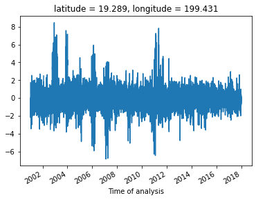
# let's remove the seasonal cycle so we can compare the data more clearly
#for ccmp data create the climatology and anomaly
ts_ccmp_climatology = ccmp_buoy.groupby('time.dayofyear').mean('time',keep_attrs=True,skipna=True)
ts_ccmp_anomaly = (ccmp_buoy.groupby('time.dayofyear')-ts_ccmp_climatology).compute()
#for buoy data create the climatology and anomaly
ts_buoy_climatology = ds_buoy.groupby('time.dayofyear').mean('time',keep_attrs=True,skipna=True)
ts_buoy_anomaly = (ds_buoy.groupby('time.dayofyear')-ts_buoy_climatology).compute()
CPU times: user 2.89 s, sys: 45.8 ms, total: 2.94 s
Wall time: 2.86 s
[16]:
%%time
#plot the data
(ts_ccmp_anomaly.wspd-ts_buoy_anomaly.wind_spd).plot()
CPU times: user 34.9 ms, sys: 47 µs, total: 35 ms
Wall time: 34.3 ms
[16]:
[<matplotlib.lines.Line2D at 0x7f32c5eb1820>]
[17]:
%%time
#calculate the mean difference and standard deviation

print('buoy minus satellite wind speeds')
rdif = (ts_buoy_anomaly.wind_spd-ts_ccmp_anomaly.wspd)
print('mean:',rdif.mean().data)
print('std:',rdif.std().data)
buoy minus satellite wind speeds
mean: -0.00028690338
std: 1.0847609043121338
CPU times: user 4.69 ms, sys: 1.16 ms, total: 5.85 ms
Wall time: 4.56 ms
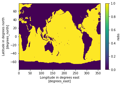
Masking satellite data and looking at frequency of low/high wind speeds.
Make a land/ocean/ice mask to show where there is actually data
Three different ways to mask the data
A daily mask that removes data with sea ice and land
sum over time for nobs (number of observations) variable
average over a month so that land and monthly sea ice are masked out
A mask that removes all data that over land or where there is ‘permanent’ sea ice
find when nobs is > 0
A climatology mask that removes all data that over land or where there has ever been sea ice
sum over time for nobs (number of observations) variable
average over a month so that land and monthly sea ice are masked out
Apply the mask
over land, CCMP is ERA5 data
for many ocean applications a land / sea ice mask is needed
below are some different mask options that use the CCMP data to generate a mask
[18]:
def mask_data(ds,type):
    if type=='daily': #daily mask removes sea ice and land
        mask_obs = ds.nobs.rolling(time=180,center=True).max('time')  #4 per day 30 days = 180 rolling window
        cutoff = 0
    if type=='land':  # land mask only (includes data over sea ice)
        mask_obs = ds.nobs.sum({'time'},keep_attrs=True)  #this will give you a LAND mask
        cutoff = 0
    if type=='climatology':  #climatology mask removes max sea ice extent and land
        test = ds.nobs.coarsen(time=16, boundary="trim").max() #subsample to every 4 days
        test = test/test #normalize
        mask_obs = test.rolling(time=10,center=True).max('time')
        mask_obs = mask_obs.sum({'time'},keep_attrs=True).compute()
        cutoff = mask_obs.sel(longitude=slice(220,230),latitude=slice(10,20)).min() #pick area in middle pacific to get #obs
        cutoff = cutoff-cutoff*.2 #just because there are some areas with a little less data eg. itcz
    dy_mask = (mask_obs>cutoff).compute()  #computing the mask speeds up subsequent operations
    masked = ds.where(dy_mask)
    return masked,dy_mask
For this tutorial we will use the climatology mask
This code will take ~10 min to run through the entire dataset to create the climatology mask
[19]:
%%time

subset = ds_ccmp.sel(time='2018')

masked,mask_obs = mask_data(subset,'climatology')

mask_obs.plot()
CPU times: user 613 ms, sys: 6.48 ms, total: 619 ms
Wall time: 3.21 s
[19]:
<matplotlib.collections.QuadMesh at 0x7f32c57c23d0>
[20]:
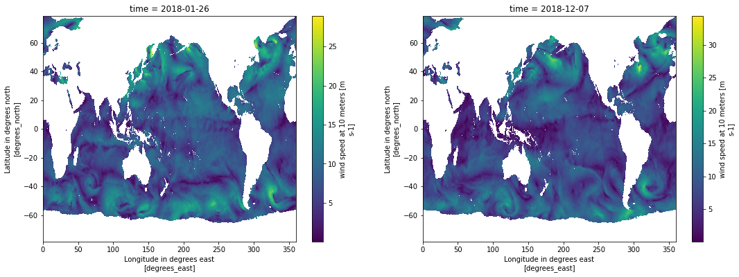
%%time

fig, ax = plt.subplots(1,2, figsize=(18,6))

masked.wspd[100,:,:].plot(ax=ax[0])

masked.wspd[-100,:,:].plot(ax=ax[1])
distributed.client - WARNING - Couldn't gather 3 keys, rescheduling {"('getitem-ea0c3fac679630cf4795077dde14fa4c', 1, 4)": (), "('getitem-ea0c3fac679630cf4795077dde14fa4c', 3, 6)": (), "('getitem-ea0c3fac679630cf4795077dde14fa4c', 1, 2)": ()}
CPU times: user 507 ms, sys: 40.6 ms, total: 548 ms
Wall time: 46.3 s
[20]:
<matplotlib.collections.QuadMesh at 0x7f32c5bcc730>
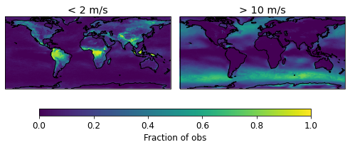
When are there low or high wind speeds at each location?
calculate percentage of low/high winds at each location
show a spatial map showing a climatology of roughness.
[21]:
%%time
from xhistogram.xarray import histogram

# wspd_bin = 0 gives fraction of winds <= 2 m/s where strong diurnal warming of the ocean surface may be present

wspd_levels = np.array([0,2,1000])

wspd_hist = histogram(subset.wspd,
                      bins=[wspd_levels],
                      dim=['time'],
                      density=False)

wspd_hist = wspd_hist/wspd_hist.sum('wspd_bin')

wspd_hist.load()
CPU times: user 175 ms, sys: 24.4 ms, total: 199 ms
Wall time: 14.2 s
[21]:
<xarray.DataArray 'histogram_wspd' (latitude: 628, longitude: 1440, wspd_bin: 2)>
array([[[0.01369863, 0.98630137],
        [0.01438356, 0.98561644],
        [0.01438356, 0.98561644],
        ...,
        [0.01506849, 0.98493151],
        [0.01506849, 0.98493151],
        [0.01369863, 0.98630137]],

       [[0.01575342, 0.98424658],
        [0.01506849, 0.98493151],
        [0.01506849, 0.98493151],
        ...,
        [0.01643836, 0.98356164],
        [0.01712329, 0.98287671],
        [0.01643836, 0.98356164]],

       [[0.01438356, 0.98561644],
        [0.01438356, 0.98561644],
        [0.01369863, 0.98630137],
        ...,
...
        ...,
        [0.0369863 , 0.9630137 ],
        [0.03767123, 0.96232877],
        [0.03630137, 0.96369863]],

       [[0.03767123, 0.96232877],
        [0.03972603, 0.96027397],
        [0.03767123, 0.96232877],
        ...,
        [0.03630137, 0.96369863],
        [0.03493151, 0.96506849],
        [0.0390411 , 0.9609589 ]],

       [[0.04041096, 0.95958904],
        [0.03835616, 0.96164384],
        [0.03835616, 0.96164384],
        ...,
        [0.04109589, 0.95890411],
        [0.04041096, 0.95958904],
        [0.04041096, 0.95958904]]])
Coordinates:
  * latitude   (latitude) float32 -78.38 -78.12 -77.88 ... 77.88 78.12 78.38
  * longitude  (longitude) float32 0.125 0.375 0.625 0.875 ... 359.4 359.6 359.9
* wspd_bin (wspd_bin) float64 1.0 501.0- latitude: 628
- longitude: 1440
- wspd_bin: 2
- 0.0137 0.9863 0.01438 0.9856 0.01438 ... 0.04041 0.9596 0.04041 0.9596
array([[[0.01369863, 0.98630137], [0.01438356, 0.98561644], [0.01438356, 0.98561644], ..., [0.01506849, 0.98493151], [0.01506849, 0.98493151], [0.01369863, 0.98630137]], [[0.01575342, 0.98424658], [0.01506849, 0.98493151], [0.01506849, 0.98493151], ..., [0.01643836, 0.98356164], [0.01712329, 0.98287671], [0.01643836, 0.98356164]], [[0.01438356, 0.98561644], [0.01438356, 0.98561644], [0.01369863, 0.98630137], ..., ... ..., [0.0369863 , 0.9630137 ], [0.03767123, 0.96232877], [0.03630137, 0.96369863]], [[0.03767123, 0.96232877], [0.03972603, 0.96027397], [0.03767123, 0.96232877], ..., [0.03630137, 0.96369863], [0.03493151, 0.96506849], [0.0390411 , 0.9609589 ]], [[0.04041096, 0.95958904], [0.03835616, 0.96164384], [0.03835616, 0.96164384], ..., [0.04109589, 0.95890411], [0.04041096, 0.95958904], [0.04041096, 0.95958904]]]) - latitude(latitude)float32-78.38 -78.12 ... 78.12 78.38
- _CoordinateAxisType :
- Lat
- _Fillvalue :
- -9999.0
- axis :
- Y
- coordinate_defines :
- center
- long_name :
- Latitude in degrees north
- standard_name :
- latitude
- units :
- degrees_north
- valid_max :
- 78.375
- valid_min :
- -78.375
array([-78.375, -78.125, -77.875, ..., 77.875, 78.125, 78.375], dtype=float32) - longitude(longitude)float320.125 0.375 0.625 ... 359.6 359.9
- _CoordinateAxisType :
- Lon
- _Fillvalue :
- -9999.0
- axis :
- X
- coordinate_defines :
- center
- long_name :
- Longitude in degrees east
- standard_name :
- longitude
- units :
- degrees_east
- valid_max :
- 359.875
- valid_min :
- 0.125
array([1.25000e-01, 3.75000e-01, 6.25000e-01, ..., 3.59375e+02, 3.59625e+02, 3.59875e+02], dtype=float32) - wspd_bin(wspd_bin)float641.0 501.0
- _Fillvalue :
- -9999.0
- height :
- 10 meters above sea-level
- long_name :
- wind speed at 10 meters
- standard_name :
- eastward_wind
- units :
- m s-1
- valid_max :
- 20.291385650634766
- valid_min :
- -21.261892318725586
array([ 1., 501.])
[22]:
%%time
from xhistogram.xarray import histogram

# wspd_bin = 1 gives fraction of winds > 10 m/s where wind speed accuracy decreases

wspd_levels = np.array([0,10,1000])
wspd_hist2 = histogram(subset.wspd,
                      bins=[wspd_levels],
                      dim=['time'],
                      density=False)

wspd_hist2 = wspd_hist2/wspd_hist2.sum('wspd_bin')

wspd_hist2.load()

whist = xr.concat([wspd_hist.isel(wspd_bin=0),wspd_hist2.isel(wspd_bin=1)],dim='wspd_bin')
CPU times: user 157 ms, sys: 27.6 ms, total: 185 ms
Wall time: 16.5 s
[23]:
%%time
#plot the data

plt.rcParams['figure.figsize'] = (8.0,4.0)
plt.rcParams.update({'font.size': 12})
fg = whist.plot(vmin=0, vmax=1,
    col="wspd_bin",
    transform=ccrs.PlateCarree(),  # remember to provide this!
    subplot_kws={
        "projection": ccrs.PlateCarree()
    },
    cbar_kwargs={"label":'Fraction of obs',"orientation": "horizontal", "shrink": 0.8, "aspect": 40},
    robust=True,
)
tstr = ['< 2 m/s','> 10 m/s']
for i, ax in enumerate(fg.axes.flat):
    ax.set_title(tstr[i])
fg.map(lambda: plt.gca().coastlines())
CPU times: user 1.5 s, sys: 387 ms, total: 1.89 s
Wall time: 1.41 s
[23]:
<xarray.plot.facetgrid.FacetGrid at 0x7f32c5c118b0>
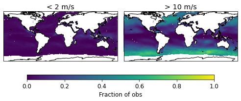
Calculate using only data over the ocean
use the mask to remove the land data
[24]:
%%time

masked = whist.where(mask_obs>0)

fg = masked.plot(vmin=0, vmax=1,
    col="wspd_bin",
    transform=ccrs.PlateCarree(),  # remember to provide this!
    subplot_kws={
        "projection": ccrs.PlateCarree()
    },
    cbar_kwargs={"label":'Fraction of obs',"orientation": "horizontal", "shrink": 0.8, "aspect": 40},
    robust=True,
)
tstr = ['< 2 m/s','> 10 m/s']
for i, ax in enumerate(fg.axes.flat):
    ax.set_title(tstr[i])
fg.map(lambda: plt.gca().coastlines())
CPU times: user 1.3 s, sys: 125 ms, total: 1.43 s
Wall time: 1.3 s
[24]:
<xarray.plot.facetgrid.FacetGrid at 0x7f32c5f2ab20>
[25]:
client.close()