
Big Arrays, Fast: Profiling Cloud Storage Read Throughput
Introduction
Many geoscience problems involve analyzing hundreds of Gigabytes (GB), many Terabytes (TB = 100 GB), or even a Petabyte (PB = 1000 TB) of data. For such data volumes, downloading data to personal computers is inefficient. Data-proximate computing, possibly using a parallel computing cluster, is one way to overcome this challenge. With data-proximate computing, a user access a remote computer which is connected tightly to shared, high-performance storage, enabling rapid processing without the need for a download step.

Figure from Data Access Modes in Science, by Ryan Abernathey. http://dx.doi.org/10.6084/M9.FIGSHARE.11987466.V1
The cloud offers many exciting new possibilities for scientific data analysis. It also brings new technical challenges. Many scientific users are accustomed to the environments found on High-Performance Computing (HPC) systems, such as NSF’s XSEDE Computers or NCAR’s Cheyenne system. These systems combine parallel computing with a high-performance shared filesystem, enabling massively parallel data analytics. When shifting workloads to the cloud, one of the biggest challenges is how to store data: cloud computing does not easily support large shared filesystems, as commonly found on HPC systems. The preferred way to store data in the cloud is using cloud object storage, such as Amazon S3 or Google Cloud Storage.
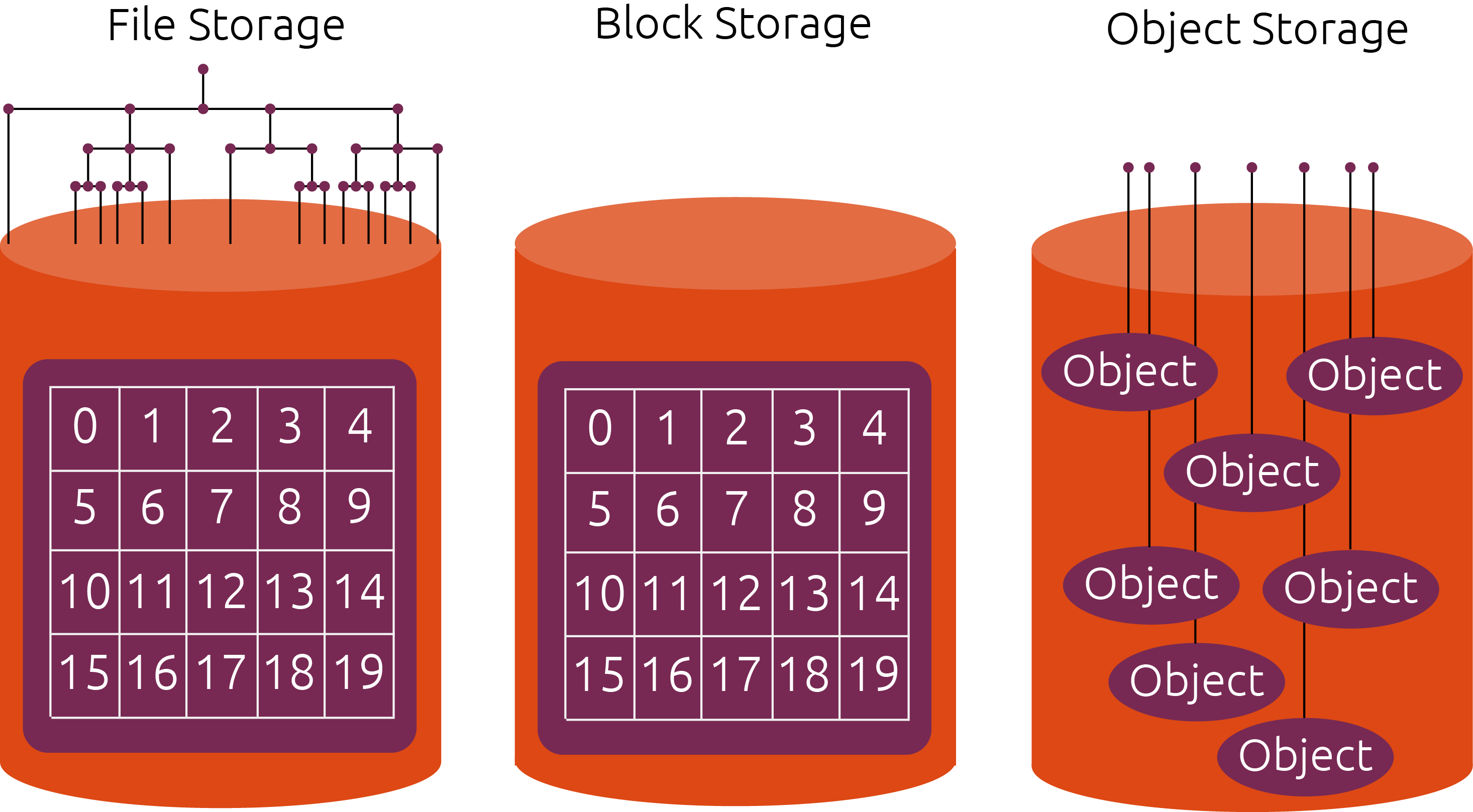
Image viaUbuntu Website, ©2020 Canonical Ltd. Ubuntu, Used with Permission
Cloud object storage is essentially a key/value storage system. They keys are strings, and the values are bytes of data. Data is read and written using HTTP calls. The performance of object storage is very different from file storage. On one hand, each individual read / write to object storage has a high overhead (10-100 ms), since it has to go over the network. On the other hand, object storage “scales out” nearly infinitely, meaning that we can make hundreds, thousands, or millions of concurrent reads / writes. This makes object storage well suited for distributed data analytics. However, the software architecture of a data analysis system must be adapted to take advantage of these properties.
The goal of this notebook is to demonstrate one software stack that can effectively exploit the scalable nature of cloud storage and computing for data processing. There are three key elements:
Zarr - a library for the storage of multi-dimensional arrays using compressed chunks.
Filesystem Spec - an abstraction layer for working with different storage technologies. Specific implementations of filesystem spec (e.g. gcsfs, Google Cloud Storage Filesystem) allow Zarr to read and write data from object storage.
Dask - a distributed computing framework that allows us to read and write data in parallel asynchronously.
Accessing the Data
For this demonstration, we will use data stored in Google Cloud Storage. The data come from the GFDL CM2.6 high-resolution climate model. They are catalogged on the Pangeo Cloud Data Catalog here:
The catalog returns an http://xarray.pydata.org/ object pointing to the data on google cloud:
[1]:
import dask.array as dsa
import fsspec
import numpy as np
import pandas as pd
from contextlib import contextmanager
import pandas as pd
import intake
import time
import seaborn as sns
import dask
from matplotlib import pyplot as plt
[2]:
from intake import open_catalog
cat = open_catalog("https://raw.githubusercontent.com/pangeo-data/pangeo-datastore/master/intake-catalogs/ocean/GFDL_CM2.6.yaml")
item = cat["GFDL_CM2_6_control_ocean"]
ds = item.to_dask()
ds
/srv/conda/envs/notebook/lib/python3.7/site-packages/xarray/coding/times.py:426: SerializationWarning: Unable to decode time axis into full numpy.datetime64 objects, continuing using cftime.datetime objects instead, reason: dates out of range
  dtype = _decode_cf_datetime_dtype(data, units, calendar, self.use_cftime)
[2]:
- nv: 2
- st_edges_ocean: 51
- st_ocean: 50
- sw_edges_ocean: 51
- sw_ocean: 50
- time: 240
- xt_ocean: 3600
- xu_ocean: 3600
- yt_ocean: 2700
- yu_ocean: 2700
- geolat_c(yu_ocean, xu_ocean)float32dask.array<chunksize=(2700, 3600), meta=np.ndarray>
- cell_methods :
- time: point
- long_name :
- uv latitude
- units :
- degrees_N
- valid_range :
- [-91.0, 91.0]
Array Chunk Bytes 38.88 MB 38.88 MB Shape (2700, 3600) (2700, 3600) Count 2 Tasks 1 Chunks Type float32 numpy.ndarray - geolat_t(yt_ocean, xt_ocean)float32dask.array<chunksize=(2700, 3600), meta=np.ndarray>
- cell_methods :
- time: point
- long_name :
- tracer latitude
- units :
- degrees_N
- valid_range :
- [-91.0, 91.0]
Array Chunk Bytes 38.88 MB 38.88 MB Shape (2700, 3600) (2700, 3600) Count 2 Tasks 1 Chunks Type float32 numpy.ndarray - geolon_c(yu_ocean, xu_ocean)float32dask.array<chunksize=(2700, 3600), meta=np.ndarray>
- cell_methods :
- time: point
- long_name :
- uv longitude
- units :
- degrees_E
- valid_range :
- [-281.0, 361.0]
Array Chunk Bytes 38.88 MB 38.88 MB Shape (2700, 3600) (2700, 3600) Count 2 Tasks 1 Chunks Type float32 numpy.ndarray - geolon_t(yt_ocean, xt_ocean)float32dask.array<chunksize=(2700, 3600), meta=np.ndarray>
- cell_methods :
- time: point
- long_name :
- tracer longitude
- units :
- degrees_E
- valid_range :
- [-281.0, 361.0]
Array Chunk Bytes 38.88 MB 38.88 MB Shape (2700, 3600) (2700, 3600) Count 2 Tasks 1 Chunks Type float32 numpy.ndarray - nv(nv)float641.0 2.0
- cartesian_axis :
- N
- long_name :
- vertex number
- units :
- none
array([1., 2.])
- st_edges_ocean(st_edges_ocean)float640.0 10.07 ... 5.29e+03 5.5e+03
- cartesian_axis :
- Z
- long_name :
- tcell zstar depth edges
- positive :
- down
- units :
- meters
array([ 0. , 10.0671 , 20.16 , 30.2889 , 40.4674 , 50.714802, 61.057499, 71.532303, 82.189903, 93.100098, 104.359703, 116.101402, 128.507599, 141.827606, 156.400208, 172.683105, 191.287704, 213.020096, 238.922699, 270.309509, 308.779297, 356.186401, 414.545685, 485.854401, 571.842773, 673.697571, 791.842773, 925.85437 , 1074.545654, 1236.186401, 1408.779297, 1590.30957 , 1778.922729, 1973.020142, 2171.287598, 2372.683105, 2576.400146, 2781.827637, 2988.507568, 3196.101562, 3404.359619, 3613.100098, 3822.189941, 4031.532227, 4241.057617, 4450.714844, 4660.467285, 4870.289062, 5080.160156, 5290.066895, 5500. ]) - st_ocean(st_ocean)float645.034 15.1 ... 5.185e+03 5.395e+03
- cartesian_axis :
- Z
- edges :
- st_edges_ocean
- long_name :
- tcell zstar depth
- positive :
- down
- units :
- meters
array([5.033550e+00, 1.510065e+01, 2.521935e+01, 3.535845e+01, 4.557635e+01, 5.585325e+01, 6.626175e+01, 7.680285e+01, 8.757695e+01, 9.862325e+01, 1.100962e+02, 1.221067e+02, 1.349086e+02, 1.487466e+02, 1.640538e+02, 1.813125e+02, 2.012630e+02, 2.247773e+02, 2.530681e+02, 2.875508e+02, 3.300078e+02, 3.823651e+02, 4.467263e+02, 5.249824e+02, 6.187031e+02, 7.286921e+02, 8.549935e+02, 9.967153e+02, 1.152376e+03, 1.319997e+03, 1.497562e+03, 1.683057e+03, 1.874788e+03, 2.071252e+03, 2.271323e+03, 2.474043e+03, 2.678757e+03, 2.884898e+03, 3.092117e+03, 3.300086e+03, 3.508633e+03, 3.717567e+03, 3.926813e+03, 4.136251e+03, 4.345864e+03, 4.555566e+03, 4.765369e+03, 4.975209e+03, 5.185111e+03, 5.395023e+03]) - sw_edges_ocean(sw_edges_ocean)float645.034 15.1 ... 5.395e+03 5.5e+03
- cartesian_axis :
- Z
- long_name :
- ucell zstar depth edges
- positive :
- down
- units :
- meters
array([5.033550e+00, 1.510065e+01, 2.521935e+01, 3.535845e+01, 4.557635e+01, 5.585325e+01, 6.626175e+01, 7.680285e+01, 8.757695e+01, 9.862325e+01, 1.100962e+02, 1.221067e+02, 1.349086e+02, 1.487466e+02, 1.640538e+02, 1.813125e+02, 2.012630e+02, 2.247773e+02, 2.530681e+02, 2.875508e+02, 3.300078e+02, 3.823651e+02, 4.467263e+02, 5.249824e+02, 6.187031e+02, 7.286921e+02, 8.549935e+02, 9.967153e+02, 1.152376e+03, 1.319997e+03, 1.497562e+03, 1.683057e+03, 1.874788e+03, 2.071252e+03, 2.271323e+03, 2.474043e+03, 2.678757e+03, 2.884898e+03, 3.092117e+03, 3.300086e+03, 3.508633e+03, 3.717567e+03, 3.926813e+03, 4.136251e+03, 4.345864e+03, 4.555566e+03, 4.765369e+03, 4.975209e+03, 5.185111e+03, 5.395023e+03, 5.500000e+03]) - sw_ocean(sw_ocean)float6410.07 20.16 ... 5.29e+03 5.5e+03
- cartesian_axis :
- Z
- edges :
- sw_edges_ocean
- long_name :
- ucell zstar depth
- positive :
- down
- units :
- meters
array([ 10.0671 , 20.16 , 30.2889 , 40.4674 , 50.714802, 61.057499, 71.532303, 82.189903, 93.100098, 104.359703, 116.101402, 128.507599, 141.827606, 156.400208, 172.683105, 191.287704, 213.020096, 238.922699, 270.309509, 308.779297, 356.186401, 414.545685, 485.854401, 571.842773, 673.697571, 791.842773, 925.85437 , 1074.545654, 1236.186401, 1408.779297, 1590.30957 , 1778.922729, 1973.020142, 2171.287598, 2372.683105, 2576.400146, 2781.827637, 2988.507568, 3196.101562, 3404.359619, 3613.100098, 3822.189941, 4031.532227, 4241.057617, 4450.714844, 4660.467285, 4870.289062, 5080.160156, 5290.066895, 5500. ]) - time(time)object0181-01-16 12:00:00 ... 0200-12-16 12:00:00
- bounds :
- time_bounds
- calendar_type :
- JULIAN
- cartesian_axis :
- T
- long_name :
- time
array([cftime.DatetimeJulian(0181-01-16 12:00:00), cftime.DatetimeJulian(0181-02-15 00:00:00), cftime.DatetimeJulian(0181-03-16 12:00:00), ..., cftime.DatetimeJulian(0200-10-16 12:00:00), cftime.DatetimeJulian(0200-11-16 00:00:00), cftime.DatetimeJulian(0200-12-16 12:00:00)], dtype=object) - xt_ocean(xt_ocean)float64-279.9 -279.8 ... 79.85 79.95
- cartesian_axis :
- X
- long_name :
- tcell longitude
- units :
- degrees_E
array([-279.95, -279.85, -279.75, ..., 79.75, 79.85, 79.95])
- xu_ocean(xu_ocean)float64-279.9 -279.8 -279.7 ... 79.9 80.0
- cartesian_axis :
- X
- long_name :
- ucell longitude
- units :
- degrees_E
array([-279.9, -279.8, -279.7, ..., 79.8, 79.9, 80. ])
- yt_ocean(yt_ocean)float64-81.11 -81.07 ... 89.94 89.98
- cartesian_axis :
- Y
- long_name :
- tcell latitude
- units :
- degrees_N
array([-81.108632, -81.066392, -81.024153, ..., 89.894417, 89.936657, 89.978896]) - yu_ocean(yu_ocean)float64-81.09 -81.05 -81.0 ... 89.96 90.0
- cartesian_axis :
- Y
- long_name :
- ucell latitude
- units :
- degrees_N
array([-81.087512, -81.045273, -81.003033, ...,  89.915537,  89.957776,
        90.      ])
- average_DT(time)timedelta64[ns]dask.array<chunksize=(12,), meta=np.ndarray>
- long_name :
- Length of average period
Array Chunk Bytes 1.92 kB 96 B Shape (240,) (12,) Count 21 Tasks 20 Chunks Type timedelta64[ns] numpy.ndarray - average_T1(time)objectdask.array<chunksize=(12,), meta=np.ndarray>
- long_name :
- Start time for average period
Array Chunk Bytes 1.92 kB 96 B Shape (240,) (12,) Count 21 Tasks 20 Chunks Type object numpy.ndarray - average_T2(time)objectdask.array<chunksize=(12,), meta=np.ndarray>
- long_name :
- End time for average period
Array Chunk Bytes 1.92 kB 96 B Shape (240,) (12,) Count 21 Tasks 20 Chunks Type object numpy.ndarray - eta_t(time, yt_ocean, xt_ocean)float32dask.array<chunksize=(3, 2700, 3600), meta=np.ndarray>
- cell_methods :
- time: mean
- long_name :
- surface height on T cells [Boussinesq (volume conserving) model]
- time_avg_info :
- average_T1,average_T2,average_DT
- units :
- meter
- valid_range :
- [-1000.0, 1000.0]
Array Chunk Bytes 9.33 GB 116.64 MB Shape (240, 2700, 3600) (3, 2700, 3600) Count 81 Tasks 80 Chunks Type float32 numpy.ndarray - eta_u(time, yu_ocean, xu_ocean)float32dask.array<chunksize=(3, 2700, 3600), meta=np.ndarray>
- cell_methods :
- time: mean
- long_name :
- surface height on U cells
- time_avg_info :
- average_T1,average_T2,average_DT
- units :
- meter
- valid_range :
- [-1000.0, 1000.0]
Array Chunk Bytes 9.33 GB 116.64 MB Shape (240, 2700, 3600) (3, 2700, 3600) Count 81 Tasks 80 Chunks Type float32 numpy.ndarray - frazil_2d(time, yt_ocean, xt_ocean)float32dask.array<chunksize=(3, 2700, 3600), meta=np.ndarray>
- cell_methods :
- time: mean
- long_name :
- ocn frazil heat flux over time step
- time_avg_info :
- average_T1,average_T2,average_DT
- units :
- W/m^2
- valid_range :
- [-10000000000.0, 10000000000.0]
Array Chunk Bytes 9.33 GB 116.64 MB Shape (240, 2700, 3600) (3, 2700, 3600) Count 81 Tasks 80 Chunks Type float32 numpy.ndarray - hblt(time, yt_ocean, xt_ocean)float32dask.array<chunksize=(3, 2700, 3600), meta=np.ndarray>
- cell_methods :
- time: mean
- long_name :
- T-cell boundary layer depth from KPP
- standard_name :
- ocean_mixed_layer_thickness_defined_by_mixing_scheme
- time_avg_info :
- average_T1,average_T2,average_DT
- units :
- m
- valid_range :
- [-100000.0, 1000000.0]
Array Chunk Bytes 9.33 GB 116.64 MB Shape (240, 2700, 3600) (3, 2700, 3600) Count 81 Tasks 80 Chunks Type float32 numpy.ndarray - ice_calving(time, yt_ocean, xt_ocean)float32dask.array<chunksize=(3, 2700, 3600), meta=np.ndarray>
- cell_methods :
- time: mean
- long_name :
- mass flux of land ice calving into ocean
- standard_name :
- water_flux_into_sea_water_from_icebergs
- time_avg_info :
- average_T1,average_T2,average_DT
- units :
- (kg/m^3)*(m/sec)
- valid_range :
- [-1000000.0, 1000000.0]
Array Chunk Bytes 9.33 GB 116.64 MB Shape (240, 2700, 3600) (3, 2700, 3600) Count 81 Tasks 80 Chunks Type float32 numpy.ndarray - mld(time, yt_ocean, xt_ocean)float32dask.array<chunksize=(3, 2700, 3600), meta=np.ndarray>
- cell_methods :
- time: mean
- long_name :
- mixed layer depth determined by density criteria
- standard_name :
- ocean_mixed_layer_thickness_defined_by_sigma_t
- time_avg_info :
- average_T1,average_T2,average_DT
- units :
- m
- valid_range :
- [0.0, 1000000.0]
Array Chunk Bytes 9.33 GB 116.64 MB Shape (240, 2700, 3600) (3, 2700, 3600) Count 81 Tasks 80 Chunks Type float32 numpy.ndarray - mld_dtheta(time, yt_ocean, xt_ocean)float32dask.array<chunksize=(3, 2700, 3600), meta=np.ndarray>
- cell_methods :
- time: mean
- long_name :
- mixed layer depth determined by temperature criteria
- time_avg_info :
- average_T1,average_T2,average_DT
- units :
- m
- valid_range :
- [0.0, 1000000.0]
Array Chunk Bytes 9.33 GB 116.64 MB Shape (240, 2700, 3600) (3, 2700, 3600) Count 81 Tasks 80 Chunks Type float32 numpy.ndarray - net_sfc_heating(time, yt_ocean, xt_ocean)float32dask.array<chunksize=(3, 2700, 3600), meta=np.ndarray>
- cell_methods :
- time: mean
- long_name :
- surface ocean heat flux coming through coupler and mass transfer
- time_avg_info :
- average_T1,average_T2,average_DT
- units :
- Watts/m^2
- valid_range :
- [-10000.0, 10000.0]
Array Chunk Bytes 9.33 GB 116.64 MB Shape (240, 2700, 3600) (3, 2700, 3600) Count 81 Tasks 80 Chunks Type float32 numpy.ndarray - pme_river(time, yt_ocean, xt_ocean)float32dask.array<chunksize=(3, 2700, 3600), meta=np.ndarray>
- cell_methods :
- time: mean
- long_name :
- mass flux of precip-evap+river via sbc (liquid, frozen, evaporation)
- standard_name :
- water_flux_into_sea_water
- time_avg_info :
- average_T1,average_T2,average_DT
- units :
- (kg/m^3)*(m/sec)
- valid_range :
- [-1000000.0, 1000000.0]
Array Chunk Bytes 9.33 GB 116.64 MB Shape (240, 2700, 3600) (3, 2700, 3600) Count 81 Tasks 80 Chunks Type float32 numpy.ndarray - pot_rho_0(time, st_ocean, yt_ocean, xt_ocean)float32dask.array<chunksize=(1, 5, 2700, 3600), meta=np.ndarray>
- cell_methods :
- time: mean
- long_name :
- potential density referenced to 0 dbar
- standard_name :
- sea_water_potential_density
- time_avg_info :
- average_T1,average_T2,average_DT
- units :
- kg/m^3
- valid_range :
- [-10.0, 100000.0]
Array Chunk Bytes 466.56 GB 194.40 MB Shape (240, 50, 2700, 3600) (1, 5, 2700, 3600) Count 2401 Tasks 2400 Chunks Type float32 numpy.ndarray - river(time, yt_ocean, xt_ocean)float32dask.array<chunksize=(3, 2700, 3600), meta=np.ndarray>
- cell_methods :
- time: mean
- long_name :
- mass flux of river (runoff + calving) entering ocean
- time_avg_info :
- average_T1,average_T2,average_DT
- units :
- (kg/m^3)*(m/sec)
- valid_range :
- [-1000000.0, 1000000.0]
Array Chunk Bytes 9.33 GB 116.64 MB Shape (240, 2700, 3600) (3, 2700, 3600) Count 81 Tasks 80 Chunks Type float32 numpy.ndarray - salt(time, st_ocean, yt_ocean, xt_ocean)float32dask.array<chunksize=(1, 5, 2700, 3600), meta=np.ndarray>
- cell_methods :
- time: mean
- long_name :
- Practical Salinity
- standard_name :
- sea_water_salinity
- time_avg_info :
- average_T1,average_T2,average_DT
- units :
- psu
- valid_range :
- [-10.0, 100.0]
Array Chunk Bytes 466.56 GB 194.40 MB Shape (240, 50, 2700, 3600) (1, 5, 2700, 3600) Count 2401 Tasks 2400 Chunks Type float32 numpy.ndarray - salt_int_rhodz(time, yt_ocean, xt_ocean)float32dask.array<chunksize=(3, 2700, 3600), meta=np.ndarray>
- cell_methods :
- time: mean
- long_name :
- vertical sum of Practical Salinity * rho_dzt
- time_avg_info :
- average_T1,average_T2,average_DT
- units :
- psu*(kg/m^3)*m
- valid_range :
- [-1.0000000200408773e+20, 1.0000000200408773e+20]
Array Chunk Bytes 9.33 GB 116.64 MB Shape (240, 2700, 3600) (3, 2700, 3600) Count 81 Tasks 80 Chunks Type float32 numpy.ndarray - sea_level(time, yt_ocean, xt_ocean)float32dask.array<chunksize=(3, 2700, 3600), meta=np.ndarray>
- cell_methods :
- time: mean
- long_name :
- effective sea level (eta_t + patm/(rho0*g)) on T cells
- standard_name :
- sea_surface_height_above_geoid
- time_avg_info :
- average_T1,average_T2,average_DT
- units :
- meter
- valid_range :
- [-1000.0, 1000.0]
Array Chunk Bytes 9.33 GB 116.64 MB Shape (240, 2700, 3600) (3, 2700, 3600) Count 81 Tasks 80 Chunks Type float32 numpy.ndarray - sea_levelsq(time, yt_ocean, xt_ocean)float32dask.array<chunksize=(3, 2700, 3600), meta=np.ndarray>
- cell_methods :
- time: mean
- long_name :
- square of effective sea level (eta_t + patm/(rho0*g)) on T cells
- standard_name :
- square_of_sea_surface_height_above_geoid
- time_avg_info :
- average_T1,average_T2,average_DT
- units :
- m^2
- valid_range :
- [-1000.0, 1000.0]
Array Chunk Bytes 9.33 GB 116.64 MB Shape (240, 2700, 3600) (3, 2700, 3600) Count 81 Tasks 80 Chunks Type float32 numpy.ndarray - sfc_hflux_coupler(time, yt_ocean, xt_ocean)float32dask.array<chunksize=(3, 2700, 3600), meta=np.ndarray>
- cell_methods :
- time: mean
- long_name :
- surface heat flux coming through coupler
- time_avg_info :
- average_T1,average_T2,average_DT
- units :
- Watts/m^2
- valid_range :
- [-10000.0, 10000.0]
Array Chunk Bytes 9.33 GB 116.64 MB Shape (240, 2700, 3600) (3, 2700, 3600) Count 81 Tasks 80 Chunks Type float32 numpy.ndarray - sfc_hflux_pme(time, yt_ocean, xt_ocean)float32dask.array<chunksize=(3, 2700, 3600), meta=np.ndarray>
- cell_methods :
- time: mean
- long_name :
- heat flux (relative to 0C) from pme transfer of water across ocean surface
- time_avg_info :
- average_T1,average_T2,average_DT
- units :
- Watts/m^2
- valid_range :
- [-10000.0, 10000.0]
Array Chunk Bytes 9.33 GB 116.64 MB Shape (240, 2700, 3600) (3, 2700, 3600) Count 81 Tasks 80 Chunks Type float32 numpy.ndarray - swflx(time, yt_ocean, xt_ocean)float32dask.array<chunksize=(3, 2700, 3600), meta=np.ndarray>
- cell_methods :
- time: mean
- long_name :
- shortwave flux into ocean (>0 heats ocean)
- standard_name :
- surface_net_downward_shortwave_flux
- time_avg_info :
- average_T1,average_T2,average_DT
- units :
- W/m^2
- valid_range :
- [-10000000000.0, 10000000000.0]
Array Chunk Bytes 9.33 GB 116.64 MB Shape (240, 2700, 3600) (3, 2700, 3600) Count 81 Tasks 80 Chunks Type float32 numpy.ndarray - tau_x(time, yu_ocean, xu_ocean)float32dask.array<chunksize=(3, 2700, 3600), meta=np.ndarray>
- cell_methods :
- time: mean
- long_name :
- i-directed wind stress forcing u-velocity
- standard_name :
- surface_downward_x_stress
- time_avg_info :
- average_T1,average_T2,average_DT
- units :
- N/m^2
- valid_range :
- [-10.0, 10.0]
Array Chunk Bytes 9.33 GB 116.64 MB Shape (240, 2700, 3600) (3, 2700, 3600) Count 81 Tasks 80 Chunks Type float32 numpy.ndarray - tau_y(time, yu_ocean, xu_ocean)float32dask.array<chunksize=(3, 2700, 3600), meta=np.ndarray>
- cell_methods :
- time: mean
- long_name :
- j-directed wind stress forcing v-velocity
- standard_name :
- surface_downward_y_stress
- time_avg_info :
- average_T1,average_T2,average_DT
- units :
- N/m^2
- valid_range :
- [-10.0, 10.0]
Array Chunk Bytes 9.33 GB 116.64 MB Shape (240, 2700, 3600) (3, 2700, 3600) Count 81 Tasks 80 Chunks Type float32 numpy.ndarray - temp(time, st_ocean, yt_ocean, xt_ocean)float32dask.array<chunksize=(1, 5, 2700, 3600), meta=np.ndarray>
- cell_methods :
- time: mean
- long_name :
- Potential temperature
- standard_name :
- sea_water_potential_temperature
- time_avg_info :
- average_T1,average_T2,average_DT
- units :
- degrees C
- valid_range :
- [-10.0, 500.0]
Array Chunk Bytes 466.56 GB 194.40 MB Shape (240, 50, 2700, 3600) (1, 5, 2700, 3600) Count 2401 Tasks 2400 Chunks Type float32 numpy.ndarray - temp_int_rhodz(time, yt_ocean, xt_ocean)float32dask.array<chunksize=(3, 2700, 3600), meta=np.ndarray>
- cell_methods :
- time: mean
- long_name :
- vertical sum of Potential temperature * rho_dzt
- time_avg_info :
- average_T1,average_T2,average_DT
- units :
- deg_C*(kg/m^3)*m
- valid_range :
- [-1.0000000200408773e+20, 1.0000000200408773e+20]
Array Chunk Bytes 9.33 GB 116.64 MB Shape (240, 2700, 3600) (3, 2700, 3600) Count 81 Tasks 80 Chunks Type float32 numpy.ndarray - temp_rivermix(time, st_ocean, yt_ocean, xt_ocean)float32dask.array<chunksize=(1, 5, 2700, 3600), meta=np.ndarray>
- cell_methods :
- time: mean
- long_name :
- cp*rivermix*rho_dzt*temp
- time_avg_info :
- average_T1,average_T2,average_DT
- units :
- Watt/m^2
- valid_range :
- [-10000000000.0, 10000000000.0]
Array Chunk Bytes 466.56 GB 194.40 MB Shape (240, 50, 2700, 3600) (1, 5, 2700, 3600) Count 2401 Tasks 2400 Chunks Type float32 numpy.ndarray - time_bounds(time, nv)timedelta64[ns]dask.array<chunksize=(12, 2), meta=np.ndarray>
- long_name :
- time axis boundaries
- calendar :
- JULIAN
Array Chunk Bytes 3.84 kB 192 B Shape (240, 2) (12, 2) Count 21 Tasks 20 Chunks Type timedelta64[ns] numpy.ndarray - ty_trans(time, st_ocean, yu_ocean, xt_ocean)float32dask.array<chunksize=(1, 5, 2700, 3600), meta=np.ndarray>
- cell_methods :
- time: mean
- long_name :
- T-cell j-mass transport
- standard_name :
- ocean_y_mass_transport
- time_avg_info :
- average_T1,average_T2,average_DT
- units :
- Sv (10^9 kg/s)
- valid_range :
- [-1.0000000200408773e+20, 1.0000000200408773e+20]
Array Chunk Bytes 466.56 GB 194.40 MB Shape (240, 50, 2700, 3600) (1, 5, 2700, 3600) Count 2401 Tasks 2400 Chunks Type float32 numpy.ndarray - u(time, st_ocean, yu_ocean, xu_ocean)float32dask.array<chunksize=(1, 5, 2700, 3600), meta=np.ndarray>
- cell_methods :
- time: mean
- long_name :
- i-current
- standard_name :
- sea_water_x_velocity
- time_avg_info :
- average_T1,average_T2,average_DT
- units :
- m/sec
- valid_range :
- [-10.0, 10.0]
Array Chunk Bytes 466.56 GB 194.40 MB Shape (240, 50, 2700, 3600) (1, 5, 2700, 3600) Count 2401 Tasks 2400 Chunks Type float32 numpy.ndarray - v(time, st_ocean, yu_ocean, xu_ocean)float32dask.array<chunksize=(1, 5, 2700, 3600), meta=np.ndarray>
- cell_methods :
- time: mean
- long_name :
- j-current
- standard_name :
- sea_water_y_velocity
- time_avg_info :
- average_T1,average_T2,average_DT
- units :
- m/sec
- valid_range :
- [-10.0, 10.0]
Array Chunk Bytes 466.56 GB 194.40 MB Shape (240, 50, 2700, 3600) (1, 5, 2700, 3600) Count 2401 Tasks 2400 Chunks Type float32 numpy.ndarray - wt(time, sw_ocean, yt_ocean, xt_ocean)float32dask.array<chunksize=(1, 50, 2700, 3600), meta=np.ndarray>
- cell_methods :
- time: mean
- long_name :
- dia-surface velocity T-points
- time_avg_info :
- average_T1,average_T2,average_DT
- units :
- m/sec
- valid_range :
- [-100000.0, 100000.0]
Array Chunk Bytes 466.56 GB 1.94 GB Shape (240, 50, 2700, 3600) (1, 50, 2700, 3600) Count 241 Tasks 240 Chunks Type float32 numpy.ndarray
- filename :
- 01810101.ocean.nc
- grid_tile :
- 1
- grid_type :
- mosaic
- title :
- CM2.6_miniBling
For this example, we are not interested in Xarray’s advanced data analytics features, so we will work directly with the raw array data. Here we examine the data from the temp variable (ocean temperature):
[3]:
data = ds.temp.data
data
[3]:
|
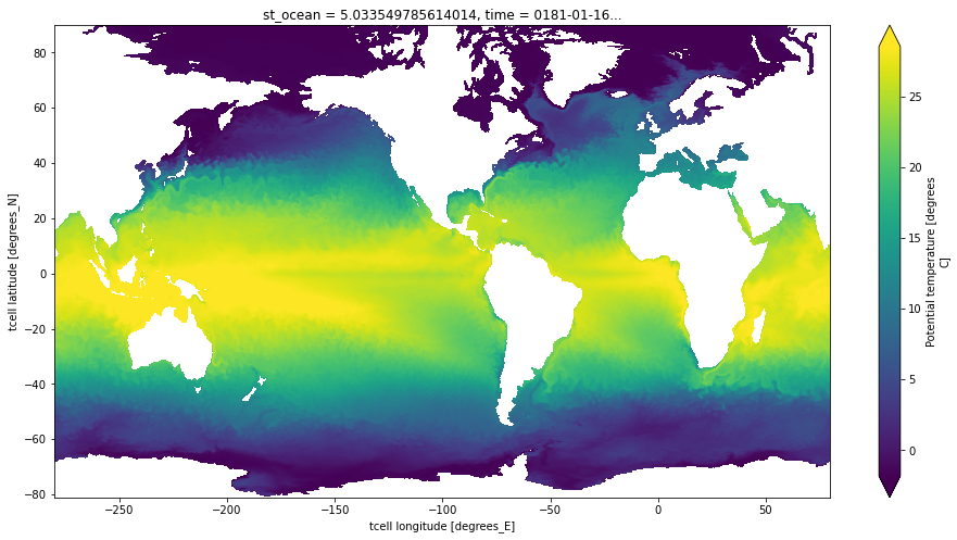
Before dropping down to the dask level, we take a quick peek at the data using Xarray’s built-in visualization capabilities.
[4]:
ds.temp[0, 0].plot(figsize=(16, 8), center=False, robust=True)
[4]:
<matplotlib.collections.QuadMesh at 0x7fe6f00e2850>
Side note: We can open this array directly with dask, bypassing xarray, if we know the path on the object store. (These give identical results.)
[5]:
item.urlpath
[5]:
'gs://cmip6/GFDL_CM2_6/control/ocean'
[6]:
dsa.from_zarr(fsspec.get_mapper("gs://cmip6/GFDL_CM2_6/control/ocean/temp"))
[6]:
|
Some important observations:
The data is organized into 2400 distinct chunks–each one corresponds to an individual object in Google Cloud Storage
The in-memory size of each chunk is 194.4 MB
The chunks are contiguous across the latitude and longitude dimensions (axes 2 and 3) and span 5 vertical levels (axis 1). Each timestep (axis 0) is in a different chunk.
Zarr + Dask know how to virtually combine these chunks into a single 4-dimensional array.
Set Up Benchmarking
Now we want to see how fast we can load data from the object store. We are not interested in any computations. Here the goal is simply to measure read performance and how it scales. In order to do this, we employ a trick: we store the data into a virtual storage target that simply discards the data, similar to piping data to /dev/null on a filesystem.
To do this, we define the following storage class:
[7]:
class DevNullStore:

    def __init__(self):
        pass

    def __setitem__(*args, **kwargs):
        pass
This is basically a dictionary that forgets whatever you put in it:
[8]:
null_store = DevNullStore()
# this line produces no error but actually does nothing
null_store['foo'] = 'bar'
Now let’s see how long it takes to store one chunk of data into this null storage target. This essentially measures the read time.
[9]:
%time dsa.store(data[0, :5], null_store, lock=False)
CPU times: user 869 ms, sys: 367 ms, total: 1.24 s
Wall time: 1.31 s
Now we want to scale this out to see how the read time scales as a function of number of parallel reads. For this, we need a Dask cluster. In our Pangeo environment, we can use Dask Gateway to create a Dask cluster. But there is an analogous way to do this on nearly any distributed computing environment. HPC-style environments (PBS, Slurm, etc.) are supported via Dask Jobqueue. Most cloud environments can work with Dask Kubernetes.
[10]:
from dask_gateway import Gateway
from dask.distributed import Client

gateway = Gateway()
cluster = gateway.new_cluster()
cluster
[11]:
client = Client(cluster)
client
[11]:
Client
|
Cluster
|
Finally we create a context manager to help us keep track of the results of our benchmarking
[12]:
class DiagnosticTimer:
    def __init__(self):
        self.diagnostics = []

    @contextmanager
    def time(self, **kwargs):
        tic = time.time()
        yield
        toc = time.time()
        kwargs["runtime"] = toc - tic
        self.diagnostics.append(kwargs)

    def dataframe(self):
        return pd.DataFrame(self.diagnostics)

diag_timer = DiagnosticTimer()
Do Benchmarking
We want to keep track of some information about our array. Here we figure out the size (in bytes) of the chunks.
[13]:
chunksize = np.prod(data.chunksize) * data.dtype.itemsize
chunksize
[13]:
194400000
And about how many workers / threads are in the cluster. The current cluster setup uses two threads and approximately 4 GB of memory per worker. These settings are the defaults for the current Pangeo environment and have not been explored extensively. We do not expect high sensitivity to these parameters here, as the task is I/O limited, not CPU limited.
[14]:
def total_nthreads():
    return sum([v for v in client.nthreads().values()])

def total_ncores():
    return sum([v for v in client.ncores().values()])

def total_workers():
    return len(client.ncores())
This is the main loop where we time a distributed read for different numbers of worker counts. We also keep track of some other metadata about our testing conditions.
[15]:
diag_kwargs = dict(nbytes=data.nbytes, chunksize=chunksize,
                   cloud='gcloud', format='zarr')


for nworkers in [30, 20, 10, 5]:
    cluster.scale(nworkers)
    time.sleep(10)
    client.wait_for_workers(nworkers)
    print(nworkers)
    with diag_timer.time(nthreads=total_nthreads(),
                         ncores=total_ncores(),
                         nworkers=total_workers(),
                         **diag_kwargs):

        future = dsa.store(data, null_store, lock=False, compute=False)
        dask.compute(future, retries=5)
30
20
10
5
[16]:
client.close()
cluster.close()
[17]:
df = diag_timer.dataframe()
df
[17]:
| nthreads | ncores | nworkers | nbytes | chunksize | cloud | format | runtime | |
|---|---|---|---|---|---|---|---|---|
| 0 | 60 | 60 | 30 | 466560000000 | 194400000 | gcloud | zarr | 117.696347 |
| 1 | 40 | 40 | 20 | 466560000000 | 194400000 | gcloud | zarr | 156.934256 |
| 2 | 20 | 20 | 10 | 466560000000 | 194400000 | gcloud | zarr | 211.342585 |
| 3 | 10 | 10 | 5 | 466560000000 | 194400000 | gcloud | zarr | 414.379612 |
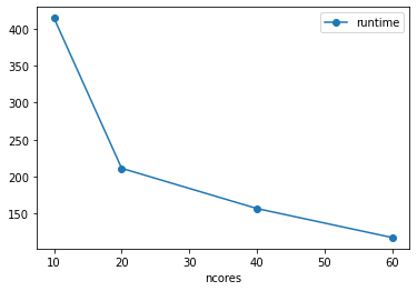
[18]:
df.plot(x='ncores', y='runtime', marker='o')
[18]:
<matplotlib.axes._subplots.AxesSubplot at 0x7fe6d935c3d0>
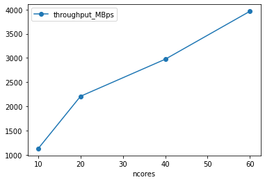
[19]:
df['throughput_MBps'] = df.nbytes / 1e6 / df['runtime']
df.plot(x='ncores', y='throughput_MBps', marker='o')
[19]:
<matplotlib.axes._subplots.AxesSubplot at 0x7fe6d90aec90>
[20]:
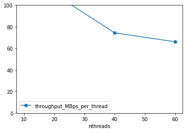
df['throughput_MBps_per_thread'] = df.throughput_MBps / df.nthreads
df.plot(x='nthreads', y='throughput_MBps_per_thread', marker='o')
plt.ylim([0, 100])
[20]:
(0.0, 100.0)
Compare Many Results
Similar tests to the one above were performed with many different cloud storage technologies and data formats:
Google Cloud Storage + Zarr Format (like the example above)
Google Cloud Storage + NetCDF Format (NetCDF files were opened directly from object storage using
gcsfsto provide file-like objects toh5py)Wasabi Cloud + Zarr Format (A discount cloud-storage vendor)
Jetstream Cloud + Zarr Format (NSF’s Cloud)
Open Storage Network (OSN) NCSA Storage Pod + Zarr Format
The NASA ECCO Data Portal (data read using
`xmitgcm.llcreader<https://xmitgcm.readthedocs.io/en/latest/llcreader.html>`__)Various OPeNDAP Servers, including:
The UCAR ESGF Node TDS Server
NOAA ESRL PSL TDS Server
The results have been archived on Zenodo: ![]()
Despite the different sources and formats, all tests were conducted in the same basic manner: 1. A “lazy” dask array referencing the source data was created 2. A dask cluster was scaled up to different sizes 3. The array was “stored” into the NullStore, forcing all data to read from the source
Note: All computing was done in Google Cloud.
[21]:
url_base = 'https://zenodo.org/record/3829032/files/'
files = {'GCS Zarr': ['gcloud-test-1.csv', 'gcloud-test-3.csv', 'gcloud-test-4.csv',
                      'gcloud-test-5.csv', 'gcloud-test-6.csv'],
         'GCS NetCDF': ['netcdf-test-1.csv'],
         'Wasabi Zarr': ['wasabi-test-1.csv', 'wasabi-test-2.csv', 'wasabi-test-3.csv'],
         'Jetstream Zarr': ['jetstream-1.csv', 'jetstream-2.csv'],
         'ECCO Data Portal': ['ecco-data-portal-1.csv', 'ecco-data-portal-2.csv'],
         'ESGF UCAR OPeNDAP': ['esgf-ucar-1.csv', 'esgf-ucar-2.csv'],
         'NOAA ESRL OPeNDAP': ['noaa-esrl-1.csv', 'noaa-esrl-2.csv'],
         'OSN Zarr': ['OSN-test-1.csv', 'OSN-test-2.csv']
        }

data = {}
for name, fnames in files.items():
    data[name] = pd.concat([pd.read_csv(f'{url_base}/{fname}') for fname in fnames])
[22]:
data['OSN Zarr']
[22]:
| Unnamed: 0 | operation | nbytes | cloud | region | nthreads | ncores | nworkers | runtime | throughput_MBps | |
|---|---|---|---|---|---|---|---|---|---|---|
| 0 | 0 | load | 466560000000 | OSN | ncsa | 52 | 52 | 26 | 81.508533 | 5724.063287 |
| 1 | 1 | load | 466560000000 | OSN | ncsa | 56 | 56 | 28 | 74.447608 | 6266.957584 |
| 2 | 2 | load | 466560000000 | OSN | ncsa | 56 | 56 | 28 | 76.227204 | 6120.649557 |
| 0 | 0 | load | 466560000000 | OSN | ncsa | 176 | 176 | 88 | 90.225218 | 5171.059835 |
| 1 | 1 | load | 466560000000 | OSN | ncsa | 176 | 176 | 88 | 87.946760 | 5305.027713 |
| 2 | 2 | load | 466560000000 | OSN | ncsa | 176 | 176 | 88 | 85.846841 | 5434.795231 |
| 3 | 3 | load | 466560000000 | OSN | ncsa | 118 | 118 | 59 | 86.004042 | 5424.861286 |
| 4 | 4 | load | 466560000000 | OSN | ncsa | 116 | 116 | 58 | 84.333328 | 5532.332396 |
| 5 | 5 | load | 466560000000 | OSN | ncsa | 56 | 56 | 28 | 78.459454 | 5946.510916 |
| 6 | 6 | load | 466560000000 | OSN | ncsa | 58 | 58 | 29 | 79.128673 | 5896.219217 |
| 7 | 7 | load | 466560000000 | OSN | ncsa | 58 | 58 | 29 | 87.597282 | 5326.192645 |
| 8 | 8 | load | 466560000000 | OSN | ncsa | 38 | 38 | 19 | 80.624812 | 5786.804199 |
| 9 | 9 | load | 466560000000 | OSN | ncsa | 36 | 36 | 18 | 88.066506 | 5297.814378 |
| 10 | 10 | load | 466560000000 | OSN | ncsa | 34 | 34 | 17 | 80.950058 | 5763.553606 |
| 11 | 11 | load | 466560000000 | OSN | ncsa | 16 | 16 | 8 | 133.425927 | 3496.771660 |
| 12 | 12 | load | 466560000000 | OSN | ncsa | 16 | 16 | 8 | 125.410473 | 3720.263469 |
| 13 | 13 | load | 466560000000 | OSN | ncsa | 18 | 18 | 9 | 121.041131 | 3854.557505 |
| 14 | 14 | load | 97200000000 | OSN | ncsa | 10 | 10 | 5 | 41.933632 | 2317.948520 |
| 15 | 15 | load | 97200000000 | OSN | ncsa | 10 | 10 | 5 | 40.639303 | 2391.773278 |
| 16 | 16 | load | 97200000000 | OSN | ncsa | 10 | 10 | 5 | 40.998851 | 2370.798158 |
| 17 | 17 | load | 38880000000 | OSN | ncsa | 4 | 4 | 2 | 54.485590 | 713.583170 |
| 18 | 18 | load | 38880000000 | OSN | ncsa | 4 | 4 | 2 | 55.811349 | 696.632509 |
| 19 | 19 | load | 38880000000 | OSN | ncsa | 4 | 4 | 2 | 52.297635 | 743.437062 |
| 20 | 20 | load | 19440000000 | OSN | ncsa | 2 | 2 | 1 | 51.179465 | 379.839847 |
| 21 | 21 | load | 19440000000 | OSN | ncsa | 2 | 2 | 1 | 44.043411 | 441.382707 |
[23]:
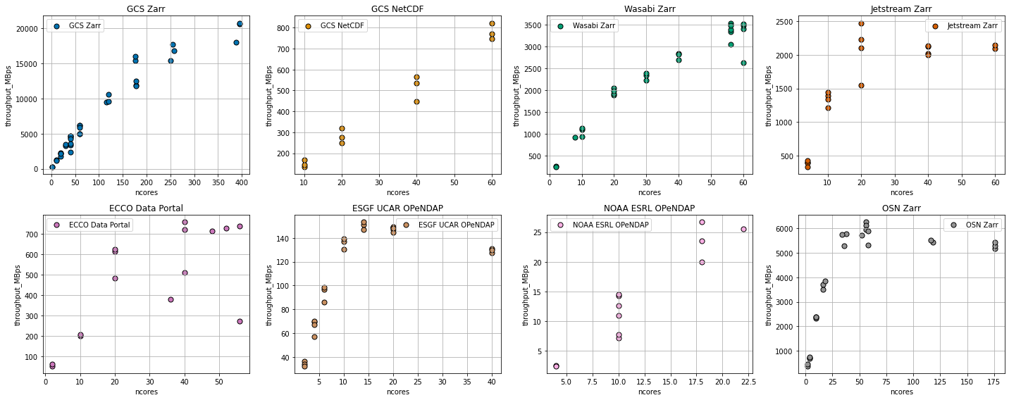
fig0, ax0 = plt.subplots()
fig1, axs = plt.subplots(nrows=2, ncols=4, figsize=(20, 8))
palette = sns.color_palette('colorblind', len(files))

for (name, df), color, ax1 in zip(data.items(), palette, axs.flat):
    for ax in [ax0, ax1]:
        df.plot(kind='scatter', x='ncores', y='throughput_MBps',
                  s=50, c=[color], edgecolor='k', ax=ax, label=name)
    ax1.grid()
    ax1.set_title(name)

ax0.grid()
ax0.legend(loc='upper left')

fig0.tight_layout()
fig1.tight_layout()
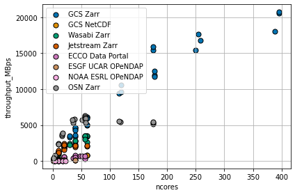
Discussion
The figure above shows a wide range of throughput rates and scaling behavior. There are a great many factors which might influence the results, including: - The structure of the source data (e.g. data format, chunk size, compression, etc.) - The rate at which the storage service can read and process data from its own disks - The transport protocol and encoding (compression, etc.) - The network bandwidth between the source and Google Cloud US-CENTRAL1 region - The overhead of the dask cluster in computing many tasks simultaneously
The comparison is far from “fair”: it is clearly biased towards Google Cloud Storage, which has optimum network proximity to the compute location. Nevertheless, we make the following observations.
Zarr is about 10x faster than NetCDF in Cloud Object Storage
Using 40 cores (20 dask workers), we were able to pull netCDF data from Google Cloud Storage at a rate of about 500 MB/s. Using the Zarr format, we could get to 5000 MB/s (5 GB/s) for the same number of dask workers.
Google Cloud Storage Scales
Both formats, however, showed good scaling, with throughput increasingly nearly linearly with the size of the cluster. The largest experiment we attempted used nearly 400 cores: we were able to pull data from GCS at roughly 20 GB/s. That’s pretty fast! At this rate, we could process a Petebyte of data in about 14 hours. However, there is a knee in the GCS-Zarr curve around 150 cores, with the scaling becoming slightly poorer above that value. We hypothesize that this is due to Dask’s overhead from handling a very large task graph.
External Cloud Storage Providers Scale…then Saturate
We tested three cloud storage providers outside of Google Cloud: Wasabi (a commercial service), Jetstream (an NSF-operated cloud), and OSN (an NSF-sponsored storage provider). These curves all show a similar pattern: good scaling for low worker counts, then a plateau. We interpret this a saturation of the network bandwidth between the data and the compute location. Of these three, Jetstream saturated at the lowest value (2 GB/s), then Wasabi (3.5 GB/s, but possibly not fully saturated yet), then OSN (5.5 GB/s). Also noteworthy is the fact that, for smaller core counts, OSN was actually faster than GCS within Google Cloud. These results are likely highly sensitive to network topology. However, they show unambiguously that OSN is an attractive choice for cloud-style storage and on-demand big-data processing.
OPeNDAP is Slow
The fastest we could get data out of an OPeNDAP server was 100 MB/s (UCAR ESGF Node). The NOAA ESRL server was more like 20 MB/s. These rates are many orders of magnitude than cloud storage. Perhaps these servers have throttling in place to limit their total bandwidth. Or perhaps the OPeNDAP protocol itself has some fundamental inefficiencies. OPeNDAP remains a very convenient protocol for remote data access; if we wish to use it for Big Data and distributed processing, data providers need to find some way to speed it up.
Conclusions
We demonstrated a protocol for testing the throughput and scalability Array data storage with the Dask computing framework. Using Google Cloud as our compute platform, we found, unsurprisingly, that a cloud-optimized storage format (Zarr), used with in-region cloud storage, provided the best raw throughput (up to 20 GB/s in our test) and scalability. We found that the same storage format also allowed us to transfer data on-demand from other clouds at reasonable rates (5 GB/s) for modest levels of parallelism. (Care must be taken in this case, however, because many cloud providers charge egress fees for data leaving their network.) Combined with Zarr, all of the cloud object storage platforms were able to deliver data orders of magnitude faster than traditional OPeNDAP servers, the standard remote-data-access protocol for the geosciences.
Future Work
This analysis could be improved in numerous ways. In the future we would like to - Investigate other cloud-native storage formats, such as TileDB and Cloud-Optimized Geotiff - Perform deeper analysis of parameter sensitivity (chunk size, compression, etc.) - Explore other clouds (e.g. AWS, Microstoft Azure)
Finally, we did not attempt to assess the relative costs associated with cloud vs. on-premises data storage, as this involves difficult questions related to total cost of ownership. However, we hope these results are useful for data providers in deciding how to provision future infrastructure for data-intensive geoscience.
Notebook Reviews
Here we include the review of the original version of this notebook and our replies.
Review 1
Evaluation of the Contribution
Overall Recommendation (100%): 9 Total points (out of 10) : 9
Comments for the Authors
“Big Arrays, Fast: Profiling Cloud Storage Read Throughput” is a good quality and, most of all, interesting science meets computer science notebook. It addresses important issues relevant to this scientific arena. The problem statement, discussion and conclusions are all compelling and pertinent to this area of inquiry.
The most important criterion “does it run” is satisfied as I was able to run the notebook to completion on https://ocean.pangeo.io (though I could not run it on Binder for some reason, “KeyError: ‘GFDL_CM2_6_control_ocean’”).
The error has been corrected in the current version.
I especially liked this notebook for the following reason:
The “computational essay” aspect receives high marks for having expository prose and computation work together to build a logical conclusion.
Figures are generated inline with matplotlib
Figures are easy to understand and interesting (e.g., the set of throughput figures at the end of the notebook).
The xarray.Dataset meta data allows for inspection via the attributes and data representation icons.
Computational cells are small and intermixed with expository prose.
Problems with this notebook:
Quite a few distracting spelling errors: Benachmarks, analagous, simultaneouslly, slighly, saturdation
Unfortunately, JupyterLab has no spell checker, a feature I have obviously become to reliant upon.
A suggestion for improvement would be to include a reference section with HTML linked DOIs for further inquiry and background material, and perhaps also a future work section.
A future work section has been included.
Review 2
Evaluation of the Contribution
Overall Recommendation (100%): 8 Total points (out of 10) : 8
Comments for the Authors
the author should add to the discussion a reason for the choice of threads, cores and workers in the ‘do benchmarking’ section
while the analysis is designed to provide a coarse grain view of the speed of zarr, it might be a valuable exercise to break the scales down to segments where they can be compared; e.g. of the four zarr tests, the n_cores scales vary from 0..400 (gcs), 0..60 (wasabi, jetstream) and 0..175 (osn) and thus these scales make it difficult to compare them when we do not have data past n_cores=60 and again n_cores=175
though the authors acknowledge the tests are not ‘fair’, indeed it would be more valuable to compare various configurations of netcdf to make such comparisons more easily interpretable
typo: change to “saturation” > We interpret this a saturdation of the network bandwidth between the data and the compute location.
the abstract should include “preliminary” to situate this work as in-progress and not a full quantitative exploration and assessment of accessing data
if at all possible the author should provide instructions for how to execute elsewhere outside the pangeo platform
licensing information as well as notebook requirements should also be provided with the notebook (or a link to the GH repo if one exists for the notebook)