Landsat-8 on AWS

• How can I efficiently find, visualize, and analyze a large set of Landsat-8 imagery on AWS?

We will examine raster images from the Landsat-8 instrument. The Landsat program is the longest-running civilian satellite imagery program, with the first satellite launched in 1972 by the US Geological Survey. Landsat 8 is the latest satellite in this program, and was launched in 2013. Landsat observations are processed into “scenes”, each of which is approximately 183 km x 170 km, with a spatial resolution of 30 meters and a temporal resolution of 16 days. The duration of the landsat program makes it an attractive source of medium-scale imagery for land surface change analyses.

This notebook is a simplified update of a blog post written in October 2018, highlighting the integration of several modern Python libraries: satsearch, intake-stac, geopandas, xarray, dask, holoviz

Finding data on the Cloud

Finding geospatial data on the Cloud has been difficult until recent years. Earth scientists are accustomed to going to specific portals to find data, for example NASA’s Earthdata Search, ESA’s Copernicus Hub (https://scihub.copernicus.eu), USGS National Map (https://www.usgs.gov/core-science-systems/national-geospatial-program/national-map). AWS has had a registry of open datasets stored on AWS for many years now https://aws.amazon.com/opendata/public-datasets/. Earth-science specific data is also listed here - https://aws.amazon.com/earth/. But what if you want to search for Landsat8 data over an area of interest? Browsing through lists of files is cumbersome.

An effort is underway to make geospatial data on the Cloud more easy to discover by having a bare-bones web-friendly and search-friendly metadata catalog standard: The SpatioTemporal Asset Catalog (STAC). Once the standard is set, many tools can co-exist to build upon it. For example https://www.element84.com/earth-search/ allows us to programmatically and visually search for data on AWS! Here we will use the satsearch Python library for searching Landsat8 on AWS. Note you could also search for Sentinel2

# Suppress library deprecation warnings
import warnings
warnings.filterwarnings('ignore')

import satsearch
print(satsearch.__version__)
print(satsearch.config.API_URL)
from satsearch import Search

0.2.3
https://earth-search-legacy.aws.element84.com

# NOTE this STAC API endpoint does not currently search the entire catalog

bbox = (-124.71, 45.47, -116.78, 48.93) #(west, south, east, north)

timeRange = '2019-01-01/2020-10-01'

# STAC metadata properties
properties =  ['eo:row=027',
               'eo:column=047',
               'landsat:tier=T1']

results = Search.search(collection='landsat-8-l1',
                        bbox=bbox,
                        datetime=timeRange,
                        property=properties,
                        sort=['<datetime'],
                        )

print('%s items' % results.found())
items = results.items()
items.save('subset.geojson')

19 items

# Remember that it is easy to load geojson with geopandas!
import geopandas as gpd

gf = gpd.read_file('subset.geojson')
gf.head()

	id	collection	eo:gsd	eo:platform	eo:instrument	eo:off_nadir	eo:bands	datetime	eo:sun_azimuth	eo:sun_elevation	eo:cloud_cover	eo:row	eo:column	landsat:product_id	landsat:scene_id	landsat:processing_level	landsat:tier	landsat:revision	eo:epsg	geometry
0	LC80470272019096	landsat-8-l1	15	landsat-8	OLI_TIRS	0	[ { "name": "B1", "common_name": "coastal", "g...	2019-04-06T19:01:20	152.713795	46.106183	79	027	047	LC08_L1TP_047027_20190406_20190422_01_T1	LC80470272019096LGN00	L1TP	T1	00	32610	POLYGON ((-124.30921 48.51312, -121.80425 48.0...
1	LC80470272019128	landsat-8-l1	15	landsat-8	OLI_TIRS	0	[ { "full_width_half_max": 0.02, "center_wavel...	2019-05-08T19:01:19	149.213545	56.592420	19	027	047	LC08_L1TP_047027_20190508_20190521_01_T1	LC80470272019128LGN00	L1TP	T1	00	32610	POLYGON ((-124.27756 48.51300, -121.77234 48.0...
2	LC80470272019160	landsat-8-l1	15	landsat-8	OLI_TIRS	0	[ { "full_width_half_max": 0.02, "center_wavel...	2019-06-09T19:01:37	143.652070	61.668260	63	027	047	LC08_L1TP_047027_20190609_20190619_01_T1	LC80470272019160LGN00	L1TP	T1	00	32610	POLYGON ((-124.28944 48.51325, -121.78398 48.0...
3	LC80470272019176	landsat-8-l1	15	landsat-8	OLI_TIRS	0	[ { "full_width_half_max": 0.02, "center_wavel...	2019-06-25T19:01:42	141.834366	61.713605	52	027	047	LC08_L1TP_047027_20190625_20190705_01_T1	LC80470272019176LGN00	L1TP	T1	00	32610	POLYGON ((-124.28314 48.51335, -121.77799 48.0...
4	LC80470272019208	landsat-8-l1	15	landsat-8	OLI_TIRS	0	[ { "full_width_half_max": 0.02, "center_wavel...	2019-07-27T19:01:51	143.987513	57.532989	76	027	047	LC08_L1TP_047027_20190727_20190801_01_T1	LC80470272019208LGN00	L1TP	T1	00	32610	POLYGON ((-124.26661 48.51255, -121.76179 48.0...

# Tidy display of band information from the 'eo:bands column'
import ast
import pandas as pd
band_info = pd.DataFrame(ast.literal_eval(gf.iloc[0]['eo:bands']))
band_info

	name	common_name	gsd	center_wavelength	full_width_half_max
0	B1	coastal	30	0.44	0.02
1	B2	blue	30	0.48	0.06
2	B3	green	30	0.56	0.06
3	B4	red	30	0.65	0.04
4	B5	nir	30	0.86	0.03
5	B6	swir16	30	1.60	0.08
6	B7	swir22	30	2.20	0.20
7	B8	pan	15	0.59	0.18
8	B9	cirrus	30	1.37	0.02
9	B10	lwir11	100	10.90	0.80
10	B11	lwir12	100	12.00	1.00

# Plot search AOI and frames on a map using Holoviz Libraries (more on these later)
import geoviews as gv
import hvplot.pandas

cols = gf.loc[:,('id','eo:row','eo:column','geometry')]

footprints = cols.hvplot(geo=True, line_color='k', hover_cols=['eo:row','eo:column'], alpha=0.1, title='Landsat 8 T1')
tiles = gv.tile_sources.CartoEco.options(width=700, height=500)
labels = gv.tile_sources.StamenLabels.options(level='annotation')
tiles * footprints * labels

ipywidgets

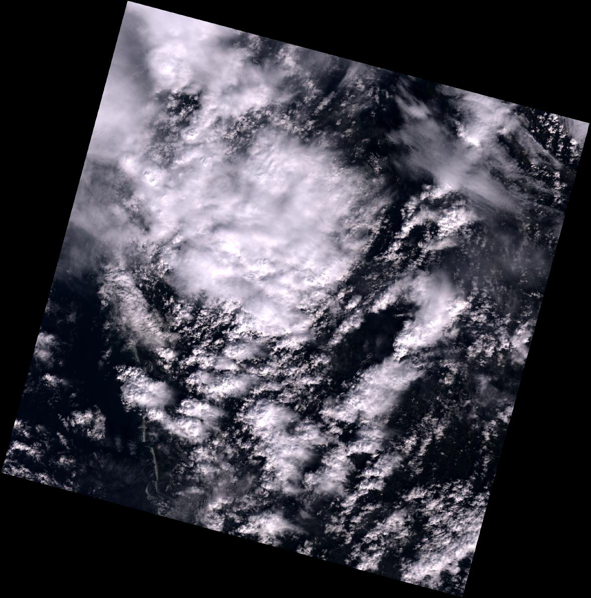
ipywidgets provide another convenient approach to custom visualizations within JupyterLab. The function below allows us to browse through all the image thumbnails for a group of images (more specifically a specific Landsat8 path and row).

from ipywidgets import interact
from IPython.display import display, Image

def browse_images(items):
    n = len(items)

    def view_image(i=0):
        item = items[i]
        print(f"id={item.id}\tdate={item.datetime}\tcloud%={item['eo:cloud_cover']}")
        display(Image(item.asset('thumbnail')['href']))

    interact(view_image, i=(0,n-1))

browse_images(items)

id=LC80470272019096     date=2019-04-06 19:01:20.935226+00:00   cloud%=79

Intake-STAC

the intake-stac library allows us to easily load these scenes described with STAC metadata into xarray DataArrays! NOTE this library is very new and will likely undergo changes in the near future. https://github.com/pangeo-data/intake-stac

# if you've installed intake-STAC, it will automatically import alongside intake
import intake
catalog = intake.open_stac_item_collection(items)

list(catalog)

['LC80470272019096',
 'LC80470272019128',
 'LC80470272019160',
 'LC80470272019176',
 'LC80470272019208',
 'LC80470272019224',
 'LC80470272019240',
 'LC80470272019272',
 'LC80470272019288',
 'LC80470272019304',
 'LC80470272019336',
 'LC80470272020003',
 'LC80470272020051',
 'LC80470272020083',
 'LC80470272020099',
 'LC80470272020131',
 'LC80470272020147',
 'LC80470272020163',
 'LC80470272020179']

sceneid = 'LC80470272019096'
catalog[sceneid]['B2'].metadata

{'type': 'image/x.geotiff',
 'eo:bands': [1],
 'title': 'Band 2 (blue)',
 'href': 'https://landsat-pds.s3.amazonaws.com/c1/L8/047/027/LC08_L1TP_047027_20190406_20190422_01_T1/LC08_L1TP_047027_20190406_20190422_01_T1_B2.TIF',
 'catalog_dir': ''}

# Let's work with the Geotiffs using Xarray
# NOTE that you don't have to specify the URL or filePath!

import xarray as xr

item = catalog[sceneid]
da = item['B2'].to_dask()
da.data

Array Chunk Bytes 125.48 MB 125.48 MB Shape (1, 7971, 7871) (1, 7971, 7871) Count 2 Tasks 1 Chunks Type uint16 numpy.ndarray

Dask Chunks and Cloud Optimized Geotiffs

Since we didn’t specify chunk sizes, everything is read as one chunk. When we load larger sets of imagery we can change these chunk sizes to use dask. It’s best to align dask chunks with the way image chunks (typically called “tiles” are stored on disk or cloud storage buckets. The landsat data is stored on AWS S3 in a tiled Geotiff format where tiles are 512x512, so we should pick som multiple of that, and typically aim for chunksizes of ~100Mb (although this is subjective). You can read more about dask chunks here: https://docs.dask.org/en/latest/array-best-practices.html

Also check out this documentation about the Cloud-optimized Geotiff format, it is an excellent choice for putting satellite raster data on Cloud storage: https://www.cogeo.org/

# Intake-STAC Item to chunked dask array
da = item.B2(chunks=dict(band=1, x=2048, y=2048)).to_dask()
da.data

Array Chunk Bytes 125.48 MB 8.39 MB Shape (1, 7971, 7871) (1, 2048, 2048) Count 17 Tasks 16 Chunks Type uint16 numpy.ndarray

# Let's load all the bands into an xarray dataset!
# Stick to bands that have the same Ground Sample Distance for simplicity
bands = band_info.query('gsd == 30').common_name.to_list()
bands

['coastal', 'blue', 'green', 'red', 'nir', 'swir16', 'swir22', 'cirrus']

stacked = item.stack_bands(bands)
da = stacked(chunks=dict(band=1, x=2048, y=2048)).to_dask()
da

<xarray.DataArray (band: 8, y: 7971, x: 7871)>
dask.array<concatenate, shape=(8, 7971, 7871), dtype=uint16, chunksize=(1, 2048, 2048), chunktype=numpy.ndarray>
Coordinates:
  * y        (y) float64 5.374e+06 5.374e+06 5.374e+06 ... 5.135e+06 5.135e+06
  * x        (x) float64 3.525e+05 3.525e+05 3.526e+05 ... 5.886e+05 5.886e+05
  * band     (band) <U2 'B1' 'B2' 'B3' 'B4' 'B5' 'B6' 'B7' 'B9'
Attributes:
    transform:      (30.0, 0.0, 352485.0, 0.0, -30.0, 5374215.0)
    crs:            +init=epsg:32610
    res:            (30.0, 30.0)
    is_tiled:       1
    nodatavals:     (nan,)
    scales:         (1.0,)
    offsets:        (0.0,)
    AREA_OR_POINT:  Point

# If we want we can convert this to an xarray dataset, with variable names corresponding to common names
# This is all very fast because we are only reading metadata
da['band'] = bands
ds = da.to_dataset(dim='band')
print('Dataset size: [Gb]', ds.nbytes/1e9)
ds

Dataset size: [Gb] 1.003962592

<xarray.Dataset>
Dimensions:  (x: 7871, y: 7971)
Coordinates:
  * y        (y) float64 5.374e+06 5.374e+06 5.374e+06 ... 5.135e+06 5.135e+06
  * x        (x) float64 3.525e+05 3.525e+05 3.526e+05 ... 5.886e+05 5.886e+05
Data variables:
    coastal  (y, x) uint16 dask.array<chunksize=(2048, 2048), meta=np.ndarray>
    blue     (y, x) uint16 dask.array<chunksize=(2048, 2048), meta=np.ndarray>
    green    (y, x) uint16 dask.array<chunksize=(2048, 2048), meta=np.ndarray>
    red      (y, x) uint16 dask.array<chunksize=(2048, 2048), meta=np.ndarray>
    nir      (y, x) uint16 dask.array<chunksize=(2048, 2048), meta=np.ndarray>
    swir16   (y, x) uint16 dask.array<chunksize=(2048, 2048), meta=np.ndarray>
    swir22   (y, x) uint16 dask.array<chunksize=(2048, 2048), meta=np.ndarray>
    cirrus   (y, x) uint16 dask.array<chunksize=(2048, 2048), meta=np.ndarray>
Attributes:
    transform:      (30.0, 0.0, 352485.0, 0.0, -30.0, 5374215.0)
    crs:            +init=epsg:32610
    res:            (30.0, 30.0)
    is_tiled:       1
    nodatavals:     (nan,)
    scales:         (1.0,)
    offsets:        (0.0,)
    AREA_OR_POINT:  Point

# Computations or visualizations trigger the streaming of bytes from S3 into memory
# Here we will compute the mean for a number of pixels for a box defined by easting and northings
zonal_mean = ds['nir'].sel(x=slice(4.99e5, 5.03e5), y=slice(5.244e6, 5.238e6)).mean()
zonal_mean.compute()

<xarray.DataArray 'nir' ()>
array(12089.203419)

Hvplot

HoloViz is a coordinated effort to make browser-based data visualization in Python easier to use, easier to learn, and more powerful! https://holoviz.org One particularly powerful library is hvplot, which allows for interactive visualizations of pandas dataframes or xarray DataArrays. With this tool you pull data on-the-fly only as required by zoom level and band selection.

import hvplot.xarray

da.hvplot.image(groupby='band', rasterize=True, dynamic=True, cmap='magma',
                width=700, height=500,  widget_location='left')

Dask-Gateway Cluster

If we don’t specify a specific cluster, dask will use the cores on the machine we are running our notebook on instead, lets connect to a Dask-Gateway cluster. You can read more about this cluster at https://gateway.dask.org/. It can take a few minutes for the cluster to become ready for computing. This is because EC2 machines are being created for you behind the scenes. Monitor the ‘Dashboard’ link to see cluster activity.

from dask_gateway import GatewayCluster
from distributed import Client

cluster = GatewayCluster()
cluster.adapt(minimum=2, maximum=20) #Keep a minimum of 2 workers, but allow for scaling up to 20 if there is RAM and CPU pressure
client = Client(cluster) #Make sure dask knows to use this cluster for computations
cluster

%%time

# First let's construct a large dataset with all the scenes in our search so that we
# have a time dimension
# Loop through geopandas geodataframe (each row is a STAC ITEM)
import dask

@dask.delayed
def stacitem_to_dataset(item):
    print(item.id)
    stacked = catalog[item.id].stack_bands(bands)
    da = stacked(chunks=dict(band=1, x=8000, y=2048)).to_dask()
    da['band'] = bands # use common names
    da = da.expand_dims(time=[pd.to_datetime(item.datetime)])
    ds = da.to_dataset(dim='band')
    return ds

lazy_datasets = []
for i,item in gf.iterrows():
    ds = stacitem_to_dataset(item)
    lazy_datasets.append(ds)

datasets = dask.compute(*lazy_datasets)

CPU times: user 87.5 ms, sys: 28.7 ms, total: 116 ms
Wall time: 50.1 s

DS = xr.concat(datasets, dim='time')

print('Dataset size: [Gb]', DS.nbytes/1e9)
DS

Dataset size: [Gb] 77.357853784

<xarray.Dataset>
Dimensions:  (time: 19, x: 7981, y: 7971)
Coordinates:
  * y        (y) float64 5.374e+06 5.374e+06 5.374e+06 ... 5.135e+06 5.135e+06
  * x        (x) float64 3.522e+05 3.522e+05 3.523e+05 ... 5.916e+05 5.916e+05
  * time     (time) datetime64[ns] 2019-04-06T19:01:20 ... 2020-06-27T19:01:35
Data variables:
    coastal  (time, y, x) float64 dask.array<chunksize=(1, 2048, 7981), meta=np.ndarray>
    blue     (time, y, x) float64 dask.array<chunksize=(1, 2048, 7981), meta=np.ndarray>
    green    (time, y, x) float64 dask.array<chunksize=(1, 2048, 7981), meta=np.ndarray>
    red      (time, y, x) float64 dask.array<chunksize=(1, 2048, 7981), meta=np.ndarray>
    nir      (time, y, x) float64 dask.array<chunksize=(1, 2048, 7981), meta=np.ndarray>
    swir16   (time, y, x) float64 dask.array<chunksize=(1, 2048, 7981), meta=np.ndarray>
    swir22   (time, y, x) float64 dask.array<chunksize=(1, 2048, 7981), meta=np.ndarray>
    cirrus   (time, y, x) float64 dask.array<chunksize=(1, 2048, 7981), meta=np.ndarray>
Attributes:
    transform:      (30.0, 0.0, 352485.0, 0.0, -30.0, 5374215.0)
    crs:            +init=epsg:32610
    res:            (30.0, 30.0)
    is_tiled:       1
    nodatavals:     (nan,)
    scales:         (1.0,)
    offsets:        (0.0,)
    AREA_OR_POINT:  Point

Distributed computations

We’ll calculate the classic NDVI index with all our data

NOTE that you should be using Landsat ARD data (https://www.usgs.gov/land-resources/nli/landsat/us-landsat-analysis-ready-data) for this with atmospheric corrections! this is just to illustrate the intuitive syntax of xarray

NDVI = (DS['nir'] - DS['red']) / (DS['nir'] + DS['red'])
NDVI

<xarray.DataArray (time: 19, y: 7971, x: 7981)>
dask.array<truediv, shape=(19, 7971, 7981), dtype=float64, chunksize=(1, 2048, 7981), chunktype=numpy.ndarray>
Coordinates:
  * y        (y) float64 5.374e+06 5.374e+06 5.374e+06 ... 5.135e+06 5.135e+06
  * x        (x) float64 3.522e+05 3.522e+05 3.523e+05 ... 5.916e+05 5.916e+05
  * time     (time) datetime64[ns] 2019-04-06T19:01:20 ... 2020-06-27T19:01:35

NDVI.data

Array Chunk Bytes 9.67 GB 130.76 MB Shape (19, 7971, 7981) (1, 2048, 7981) Count 3129 Tasks 76 Chunks Type float64 numpy.ndarray

A note on distributed versus local memory

#ndvi_my_memory = NDVI.compute() # compute pulls computation results into notebook process
NDVI = NDVI.persist() # persist keeps computation results on the dask cluster

# Plotting pulls data from distributed cluster memory on-demand
NDVI.hvplot.image(groupby='time', x='x',y='y',
                  cmap='BrBG', clim=(-1,1),
                  rasterize=True, dynamic=True,
                  width=700, height=500)

# Grab a subset and save as a netcdf file
sub = NDVI.sel(x=slice(4.5e5,5.0e5), y=slice(5.25e6,5.2e6)).mean(dim=['time'])
sub.hvplot.image(rasterize=True, dynamic=True, width=700, height=500, cmap='greens')

myda = sub.compute() #pull subset to local memory first, some formats allow distributed writing too
myda.to_netcdf(path='myndvi.nc', engine='h5netcdf')

round_trip = xr.load_dataarray('myndvi.nc')

round_trip

<xarray.DataArray (y: 1667, x: 1667)>
array([[0.18563007, 0.19059552, 0.19488273, ..., 0.22227457, 0.22484207,
        0.22228028],
       [0.19064889, 0.19709001, 0.1931438 , ..., 0.2119117 , 0.21135045,
        0.2102868 ],
       [0.18888327, 0.18884146, 0.17802309, ..., 0.21959484, 0.22006417,
        0.21836583],
       ...,
       [0.07520521, 0.09875064, 0.11840775, ..., 0.19892638, 0.22551886,
        0.25085544],
       [0.06189936, 0.13935029, 0.14722115, ..., 0.23731821, 0.24823126,
        0.25648183],
       [0.08428243, 0.13998925, 0.18112026, ..., 0.25152911, 0.25269817,
        0.25897627]])
Coordinates:
  * x        (x) float64 4.5e+05 4.5e+05 4.501e+05 ... 4.999e+05 5e+05 5e+05
  * y        (y) float64 5.25e+06 5.25e+06 5.25e+06 ... 5.2e+06 5.2e+06 5.2e+06

# Be a good citizen and always explicitly shut down computing resources when you're not using them!
# client.close()
# cluster.close()