Reproducing Key Figures from Kay et al. (2015) Paper

Introduction

This Jupyter Notebook demonstrates how one might use the NCAR Community Earth System Model (CESM) Large Ensemble (LENS) data hosted on AWS S3 (doi:10.26024/wt24-5j82). The notebook shows how to reproduce figures 2 and 4 from the Kay et al. (2015) paper describing the CESM LENS dataset (doi:10.1175/BAMS-D-13-00255.1)

This resource is intended to be helpful for people not familiar with elements of the Pangeo framework including Jupyter Notebooks, Xarray, and Zarr data format, or with the original paper, so it includes additional explanation.

Set up environment

# Display output of plots directly in Notebook
%matplotlib inline
import warnings
warnings.filterwarnings("ignore")

import intake
import numpy as np
import pandas as pd
import xarray as xr

Create and Connect to Dask Distributed Cluster

# Create cluster
from dask_gateway import Gateway
from dask.distributed import Client
gateway = Gateway()
cluster = gateway.new_cluster()
cluster.adapt(minimum=2, maximum=100)
# Connect to cluster
client = Client(cluster)
# Display cluster dashboard URL
cluster

☝️ Link to scheduler dashboard will appear above.

Load data into xarray from a catalog using intake-esm

• Intake-esm Documentation

# Open collection description file
catalog_url = 'https://ncar-cesm-lens.s3-us-west-2.amazonaws.com/catalogs/aws-cesm1-le.json'
col = intake.open_esm_datastore(catalog_url)
col

aws-cesm1-le catalog with 56 dataset(s) from 409 asset(s):

	unique
component	5
frequency	6
experiment	4
variable	65
path	394
variable_long_name	62
dim_per_tstep	3
start	13
end	12

# Show the first few lines of the catalog
col.df.head(10)

	component	frequency	experiment	variable	path	variable_long_name	dim_per_tstep	start	end
0	atm	daily	20C	FLNS	s3://ncar-cesm-lens/atm/daily/cesmLE-20C-FLNS....	net longwave flux at surface	2.0	1920-01-01 12:00:00	2005-12-30 12:00:00
1	atm	daily	20C	FLNSC	s3://ncar-cesm-lens/atm/daily/cesmLE-20C-FLNSC...	clearsky net longwave flux at surface	2.0	1920-01-01 12:00:00	2005-12-30 12:00:00
2	atm	daily	20C	FLUT	s3://ncar-cesm-lens/atm/daily/cesmLE-20C-FLUT....	upwelling longwave flux at top of model	2.0	1920-01-01 12:00:00	2005-12-30 12:00:00
3	atm	daily	20C	FSNS	s3://ncar-cesm-lens/atm/daily/cesmLE-20C-FSNS....	net solar flux at surface	2.0	1920-01-01 12:00:00	2005-12-30 12:00:00
4	atm	daily	20C	FSNSC	s3://ncar-cesm-lens/atm/daily/cesmLE-20C-FSNSC...	clearsky net solar flux at surface	2.0	1920-01-01 12:00:00	2005-12-30 12:00:00
5	atm	daily	20C	FSNTOA	s3://ncar-cesm-lens/atm/daily/cesmLE-20C-FSNTO...	net solar flux at top of atmosphere	2.0	1920-01-01 12:00:00	2005-12-30 12:00:00
6	atm	daily	20C	ICEFRAC	s3://ncar-cesm-lens/atm/daily/cesmLE-20C-ICEFR...	fraction of sfc area covered by sea-ice	2.0	1920-01-01 12:00:00	2005-12-30 12:00:00
7	atm	daily	20C	LHFLX	s3://ncar-cesm-lens/atm/daily/cesmLE-20C-LHFLX...	surface latent heat flux	2.0	1920-01-01 12:00:00	2005-12-30 12:00:00
8	atm	daily	20C	PRECL	s3://ncar-cesm-lens/atm/daily/cesmLE-20C-PRECL...	large-scale (stable) precipitation rate (liq +...	2.0	1920-01-01 12:00:00	2005-12-30 12:00:00
9	atm	daily	20C	PRECSC	s3://ncar-cesm-lens/atm/daily/cesmLE-20C-PRECS...	convective snow rate (water equivalent)	2.0	1920-01-01 12:00:00	2005-12-30 12:00:00

# Show expanded version of collection structure with details
import pprint
uniques = col.unique(columns=["component", "frequency", "experiment", "variable"])
pprint.pprint(uniques, compact=True, indent=4)

{   'component': {   'count': 5,
                     'values': ['atm', 'ice_nh', 'ice_sh', 'lnd', 'ocn']},
    'experiment': {'count': 4, 'values': ['20C', 'CTRL', 'HIST', 'RCP85']},
    'frequency': {   'count': 6,
                     'values': [   'daily', 'hourly6-1990-2005',
                                   'hourly6-2026-2035', 'hourly6-2071-2080',
                                   'monthly', 'static']},
    'variable': {   'count': 65,
                    'values': [   'DIC', 'DOC', 'FLNS', 'FLNSC', 'FLUT', 'FSNO',
                                  'FSNS', 'FSNSC', 'FSNTOA', 'FW', 'H2OSNO',
                                  'HMXL', 'ICEFRAC', 'LHFLX', 'O2', 'PD',
                                  'PRECC', 'PRECL', 'PRECSC', 'PRECSL', 'PSL',
                                  'Q', 'QFLUX', 'QRUNOFF', 'QSW_HBL', 'QSW_HTP',
                                  'RAIN', 'RESID_S', 'SALT', 'SFWF',
                                  'SFWF_WRST', 'SHF', 'SHFLX', 'SHF_QSW',
                                  'SNOW', 'SOILLIQ', 'SOILWATER_10CM', 'SSH',
                                  'SST', 'T', 'TAUX', 'TAUX2', 'TAUY', 'TAUY2',
                                  'TEMP', 'TMQ', 'TREFHT', 'TREFHTMN',
                                  'TREFHTMX', 'TS', 'U', 'UES', 'UET', 'UVEL',
                                  'VNS', 'VNT', 'VVEL', 'WTS', 'WTT', 'WVEL',
                                  'Z3', 'aice', 'aice_d', 'hi', 'hi_d']}}

Extract data needed to construct Figure 2 of Kay et al. paper

Search the catalog to find the desired data, in this case the reference height temperature of the atmosphere, at daily time resolution, for the Historical, 20th Century, and RCP8.5 (IPCC Representative Concentration Pathway 8.5) experiments

col_subset = col.search(frequency=["daily", "monthly"], component="atm", variable="TREFHT",
                        experiment=["20C", "RCP85", "HIST"])

col_subset

aws-cesm1-le catalog with 6 dataset(s) from 6 asset(s):

	unique
component	1
frequency	2
experiment	3
variable	1
path	6
variable_long_name	1
dim_per_tstep	2
start	6
end	6

col_subset.df

	component	frequency	experiment	variable	path	variable_long_name	dim_per_tstep	start	end
0	atm	daily	20C	TREFHT	s3://ncar-cesm-lens/atm/daily/cesmLE-20C-TREFH...	reference height temperature	2.0	1920-01-01 12:00:00	2005-12-30 12:00:00
1	atm	daily	HIST	TREFHT	s3://ncar-cesm-lens/atm/daily/cesmLE-HIST-TREF...	reference height temperature	1.0	1850-01-01 00:00:00	1919-12-31 12:00:00
2	atm	daily	RCP85	TREFHT	s3://ncar-cesm-lens/atm/daily/cesmLE-RCP85-TRE...	reference height temperature	2.0	2006-01-01 12:00:00	2100-12-31 12:00:00
3	atm	monthly	20C	TREFHT	s3://ncar-cesm-lens/atm/monthly/cesmLE-20C-TRE...	reference height temperature	2.0	1920-01-16 12:00:00	2005-12-16 12:00:00
4	atm	monthly	HIST	TREFHT	s3://ncar-cesm-lens/atm/monthly/cesmLE-HIST-TR...	reference height temperature	1.0	1850-01-16 12:00:00	1919-12-16 12:00:00
5	atm	monthly	RCP85	TREFHT	s3://ncar-cesm-lens/atm/monthly/cesmLE-RCP85-T...	reference height temperature	2.0	2006-01-16 12:00:00	2100-12-16 12:00:00

# Load catalog entries for subset into a dictionary of xarray datasets
dsets = col_subset.to_dataset_dict(zarr_kwargs={"consolidated": True}, storage_options={"anon": True})
print(f"\nDataset dictionary keys:\n {dsets.keys()}")

--> The keys in the returned dictionary of datasets are constructed as follows:
        'component.experiment.frequency'

100.00% [6/6 00:05<00:00]

Dataset dictionary keys:
 dict_keys(['atm.RCP85.monthly', 'atm.20C.monthly', 'atm.HIST.daily', 'atm.RCP85.daily', 'atm.20C.daily', 'atm.HIST.monthly'])

# Define Xarray datasets corresponding to the three experiments
ds_HIST = dsets['atm.HIST.monthly']
ds_20C = dsets['atm.20C.daily']
ds_RCP85 = dsets['atm.RCP85.daily']

# Use Dask.Distributed utility function to display size of each dataset
from distributed.utils import format_bytes
print(f"Historical: {format_bytes(ds_HIST.nbytes)}\n"
      f"20th Century: {format_bytes(ds_20C.nbytes)}\n"
      f"RCP8.5: {format_bytes(ds_RCP85.nbytes)}")

Historical: 185.82 MB
20th Century: 277.71 GB
RCP8.5: 306.78 GB

# Extract the Reference Height Temperature data variable
t_hist = ds_HIST["TREFHT"]
t_20c = ds_20C["TREFHT"]
t_rcp = ds_RCP85["TREFHT"]
t_20c

<xarray.DataArray 'TREFHT' (member_id: 40, time: 31389, lat: 192, lon: 288)>
dask.array<zarr, shape=(40, 31389, 192, 288), dtype=float32, chunksize=(1, 576, 192, 288), chunktype=numpy.ndarray>
Coordinates:
  * lat        (lat) float64 -90.0 -89.06 -88.12 -87.17 ... 88.12 89.06 90.0
  * lon        (lon) float64 0.0 1.25 2.5 3.75 5.0 ... 355.0 356.2 357.5 358.8
  * member_id  (member_id) int64 1 2 3 4 5 6 7 8 ... 34 35 101 102 103 104 105
  * time       (time) object 1920-01-01 12:00:00 ... 2005-12-30 12:00:00
Attributes:
    cell_methods:  time: mean
    long_name:     Reference height temperature
    units:         K

# The global surface temperature anomaly was computed relative to the 1961-90 base period
# in the Kay et al. paper, so extract that time slice
t_ref = t_20c.sel(time=slice("1961", "1990"))

Read grid cell areas

Cell size varies with latitude, so this must be accounted for when computing the global mean.

cat = col.search(frequency="static", component="atm", experiment=["20C"])
_, grid = cat.to_dataset_dict(aggregate=False, zarr_kwargs={"consolidated": True}).popitem()
grid

--> The keys in the returned dictionary of datasets are constructed as follows:
        'component.frequency.experiment.variable.path.variable_long_name.dim_per_tstep.start.end'

100.00% [1/1 00:00<00:00]

<xarray.Dataset>
Dimensions:   (bnds: 2, ilev: 31, lat: 192, lev: 30, lon: 288, slat: 191, slon: 288)
Coordinates:
    P0        float64 ...
    area      (lat, lon) float32 dask.array<chunksize=(192, 288), meta=np.ndarray>
    gw        (lat) float64 dask.array<chunksize=(192,), meta=np.ndarray>
    hyai      (ilev) float64 dask.array<chunksize=(31,), meta=np.ndarray>
    hyam      (lev) float64 dask.array<chunksize=(30,), meta=np.ndarray>
    hybi      (ilev) float64 dask.array<chunksize=(31,), meta=np.ndarray>
    hybm      (lev) float64 dask.array<chunksize=(30,), meta=np.ndarray>
  * ilev      (ilev) float64 2.255 5.032 10.16 18.56 ... 947.4 967.5 985.1 1e+03
  * lat       (lat) float64 -90.0 -89.06 -88.12 -87.17 ... 88.12 89.06 90.0
    lat_bnds  (lat, bnds) float64 dask.array<chunksize=(192, 2), meta=np.ndarray>
  * lev       (lev) float64 3.643 7.595 14.36 24.61 ... 936.2 957.5 976.3 992.6
  * lon       (lon) float64 0.0 1.25 2.5 3.75 5.0 ... 355.0 356.2 357.5 358.8
    lon_bnds  (lon, bnds) float64 dask.array<chunksize=(288, 2), meta=np.ndarray>
    ntrk      int32 ...
    ntrm      int32 ...
    ntrn      int32 ...
  * slat      (slat) float64 -89.53 -88.59 -87.64 -86.7 ... 87.64 88.59 89.53
  * slon      (slon) float64 -0.625 0.625 1.875 3.125 ... 355.6 356.9 358.1
    w_stag    (slat) float64 dask.array<chunksize=(191,), meta=np.ndarray>
    wnummax   (lat) int32 dask.array<chunksize=(192,), meta=np.ndarray>
Dimensions without coordinates: bnds
Data variables:
    *empty*
Attributes:
    intake_esm_dataset_key:  atm.static.20C.nan.s3://ncar-cesm-lens/atm/stati...

cell_area = grid.area.load()
total_area = cell_area.sum()
cell_area

<xarray.DataArray 'area' (lat: 192, lon: 288)>
array([[2.994837e+07, 2.994837e+07, 2.994837e+07, ..., 2.994837e+07,
        2.994837e+07, 2.994837e+07],
       [2.395748e+08, 2.395748e+08, 2.395748e+08, ..., 2.395748e+08,
        2.395748e+08, 2.395748e+08],
       [4.790848e+08, 4.790848e+08, 4.790848e+08, ..., 4.790848e+08,
        4.790848e+08, 4.790848e+08],
       ...,
       [4.790848e+08, 4.790848e+08, 4.790848e+08, ..., 4.790848e+08,
        4.790848e+08, 4.790848e+08],
       [2.395748e+08, 2.395748e+08, 2.395748e+08, ..., 2.395748e+08,
        2.395748e+08, 2.395748e+08],
       [2.994837e+07, 2.994837e+07, 2.994837e+07, ..., 2.994837e+07,
        2.994837e+07, 2.994837e+07]], dtype=float32)
Coordinates:
    P0       float64 1e+05
    area     (lat, lon) float32 29948370.0 29948370.0 ... 29948370.0 29948370.0
    gw       (lat) float64 3.382e-05 nan nan nan nan ... nan nan nan 3.382e-05
  * lat      (lat) float64 -90.0 -89.06 -88.12 -87.17 ... 87.17 88.12 89.06 90.0
  * lon      (lon) float64 0.0 1.25 2.5 3.75 5.0 ... 355.0 356.2 357.5 358.8
    ntrk     int32 1
    ntrm     int32 1
    ntrn     int32 1
    wnummax  (lat) int32 1 -2147483648 -2147483648 ... -2147483648 -2147483648 1
Attributes:
    long_name:      Grid-Cell Area
    standard_name:  cell_area
    units:          m2

Define weighted means

Note: resample(time="AS") does an Annual resampling based on Start of calendar year.

See documentation for Pandas resampling options

t_ref_ts = (
    (t_ref.resample(time="AS").mean("time") * cell_area).sum(dim=("lat", "lon"))
    / total_area
).mean(dim=("time", "member_id"))

t_hist_ts = (
    (t_hist.resample(time="AS").mean("time") * cell_area).sum(dim=("lat", "lon"))
) / total_area

t_20c_ts = (
    (t_20c.resample(time="AS").mean("time") * cell_area).sum(dim=("lat", "lon"))
) / total_area

t_rcp_ts = (
    (t_rcp.resample(time="AS").mean("time") * cell_area).sum(dim=("lat", "lon"))
) / total_area

Read data and compute means

Note: Dask’s “lazy execution” philosophy means that until this point we have not actually read the bulk of the data. These steps take a while to complete, so we include the Notebook “cell magic” directive %%time to display elapsed and CPU times after computation.

%%time
t_ref_mean = t_ref_ts.load()
t_ref_mean

CPU times: user 4.22 s, sys: 84.4 ms, total: 4.31 s
Wall time: 56.6 s

<xarray.DataArray ()>
array(286.38766, dtype=float32)
Coordinates:
    P0       float64 1e+05
    ntrk     int32 1
    ntrm     int32 1
    ntrn     int32 1

%%time
t_hist_ts_df = t_hist_ts.to_series().T
t_hist_ts_df.head()

CPU times: user 227 ms, sys: 7.45 ms, total: 235 ms
Wall time: 2.47 s

time
1850-01-01 00:00:00    286.205444
1851-01-01 00:00:00    286.273590
1852-01-01 00:00:00    286.248016
1853-01-01 00:00:00    286.240753
1854-01-01 00:00:00    286.150757
dtype: float32

%%time
t_20c_ts_df = t_20c_ts.to_series().unstack().T
t_20c_ts_df.head()

distributed.client - WARNING - Couldn't gather 2 keys, rescheduling {"('truediv-b953cf0d57c0846bc584c86a2f3a3dcb', 20, 83)": (), "('truediv-b953cf0d57c0846bc584c86a2f3a3dcb', 6, 11)": ()}

CPU times: user 13 s, sys: 457 ms, total: 13.4 s
Wall time: 2min 17s

member_id	1	2	3	4	5	6	7	8	9	10	...	31	32	33	34	35	101	102	103	104	105
time
1920-01-01 00:00:00	286.311676	286.346863	286.283936	286.365051	286.328400	286.374512	286.387177	286.302338	286.376007	286.348663	...	286.243713	286.283813	286.174377	286.309479	286.297028	286.342316	286.342346	286.378021	286.322083	286.255188
1921-01-01 00:00:00	286.249603	286.198578	286.287506	286.390289	286.309784	286.334747	286.309937	286.300873	286.314240	286.306244	...	286.178558	286.316467	286.073853	286.296082	286.317352	286.374298	286.246185	286.355591	286.493042	286.224823
1922-01-01 00:00:00	286.293854	286.296844	286.265747	286.336914	286.293915	286.218872	286.010254	286.195770	286.205841	286.396942	...	286.143463	286.316132	286.140900	286.294434	286.327911	286.142883	286.413239	286.368683	286.502197	286.281860
1923-01-01 00:00:00	286.327942	286.321838	286.251160	286.322327	286.236725	286.151855	286.066864	286.203583	286.271698	286.291260	...	286.168610	286.300781	286.096191	286.115479	286.227142	286.226837	286.512238	286.381165	286.215485	286.396912
1924-01-01 00:00:00	286.308380	286.238281	286.147858	286.311798	286.362732	286.185822	286.249084	286.288116	286.330627	286.411957	...	286.142395	286.287109	286.233795	286.201202	286.253906	286.323425	286.255035	286.221741	286.247589	286.421387

5 rows × 40 columns

%%time
t_rcp_ts_df = t_rcp_ts.to_series().unstack().T
t_rcp_ts_df.head()

CPU times: user 13.9 s, sys: 299 ms, total: 14.2 s
Wall time: 1min 18s

member_id	1	2	3	4	5	6	7	8	9	10	...	31	32	33	34	35	101	102	103	104	105
time
2006-01-01 00:00:00	286.764832	286.960358	286.679230	286.793152	286.754547	287.022339	286.850464	287.089844	286.960022	286.775787	...	286.866089	286.925049	286.663971	286.955414	286.712524	287.115601	286.863556	286.881683	287.308411	287.030334
2007-01-01 00:00:00	287.073792	286.908539	286.808746	286.998901	286.841675	286.993042	286.914124	286.938965	286.933563	286.675385	...	286.804108	286.849548	286.628204	287.010529	286.811554	287.187225	286.862823	287.008270	287.222534	287.239044
2008-01-01 00:00:00	287.104095	286.815033	286.995056	287.081543	287.100708	286.960510	286.854706	286.878937	287.062927	286.702454	...	286.825653	286.844086	286.811859	286.803741	286.956635	287.080994	286.930084	286.945801	287.087128	287.157745
2009-01-01 00:00:00	286.984497	287.059448	287.010498	287.144714	286.948700	287.092316	286.888458	287.050934	287.138428	286.890839	...	286.785797	286.876556	286.953094	287.060364	287.056946	287.124908	287.005615	287.083984	287.254211	287.060730
2010-01-01 00:00:00	286.991821	287.102295	286.988129	286.875183	286.954407	287.121796	286.938843	287.116211	286.957245	287.049622	...	286.937317	286.928314	286.980499	287.118713	287.178040	287.030212	287.114716	287.083038	287.256927	287.066528

5 rows × 40 columns

Get observations for figure 2 (HadCRUT4; Morice et al. 2012)

# Observational time series data for comparison with ensemble average
obsDataURL = "https://www.esrl.noaa.gov/psd/thredds/dodsC/Datasets/cru/hadcrut4/air.mon.anom.median.nc"

ds = xr.open_dataset(obsDataURL).load()
ds

<xarray.Dataset>
Dimensions:    (lat: 36, lon: 72, nbnds: 2, time: 2046)
Coordinates:
  * lat        (lat) float32 87.5 82.5 77.5 72.5 ... -72.5 -77.5 -82.5 -87.5
  * lon        (lon) float32 -177.5 -172.5 -167.5 -162.5 ... 167.5 172.5 177.5
  * time       (time) datetime64[ns] 1850-01-01 1850-02-01 ... 2020-06-01
Dimensions without coordinates: nbnds
Data variables:
    time_bnds  (time, nbnds) datetime64[ns] 1850-01-01 1850-01-31 ... 2020-06-30
    air        (time, lat, lon) float32 nan nan nan nan nan ... nan nan nan nan
Attributes:
    platform:                        Surface
    title:                           HADCRUT4 Combined Air Temperature/SST An...
    history:                         Originally created at NOAA/ESRL PSD by C...
    Conventions:                     CF-1.0
    Comment:                         This dataset supersedes V3
    Source:                          Obtained from http://hadobs.metoffice.co...
    version:                         4.2.0
    dataset_title:                   HadCRUT4
    References:                      https://www.psl.noaa.gov/data/gridded/da...
    DODS_EXTRA.Unlimited_Dimension:  time

def weighted_temporal_mean(ds):
    """
    weight by days in each month
    """
    time_bound_diff = ds.time_bnds.diff(dim="nbnds")[:, 0]
    wgts = time_bound_diff.groupby("time.year") / time_bound_diff.groupby(
        "time.year"
    ).sum(xr.ALL_DIMS)
    np.testing.assert_allclose(wgts.groupby("time.year").sum(xr.ALL_DIMS), 1.0)
    obs = ds["air"]
    cond = obs.isnull()
    ones = xr.where(cond, 0.0, 1.0)
    obs_sum = (obs * wgts).resample(time="AS").sum(dim="time")
    ones_out = (ones * wgts).resample(time="AS").sum(dim="time")
    obs_s = (obs_sum / ones_out).mean(("lat", "lon")).to_series()
    return obs_s

• Limit Observations to 20th Century

obs_s = weighted_temporal_mean(ds)
obs_s = obs_s['1920':]
obs_s.head()

time
1920-01-01   -0.262006
1921-01-01   -0.195891
1922-01-01   -0.301986
1923-01-01   -0.269062
1924-01-01   -0.292857
Freq: AS-JAN, dtype: float64

all_ts_anom = pd.concat([t_20c_ts_df, t_rcp_ts_df]) - t_ref_mean.data
years = [val.year for val in all_ts_anom.index]
obs_years = [val.year for val in obs_s.index]

# Combine ensemble member 1 data from historical and 20th century experiments
hist_anom = t_hist_ts_df - t_ref_mean.data
member1 = pd.concat([hist_anom.iloc[:-2], all_ts_anom.iloc[:,0]], verify_integrity=True)
member1_years = [val.year for val in member1.index]

Figure 2: Global surface temperature anomaly (1961-90 base period) for individual ensemble members, and observations

import matplotlib.pyplot as plt

ax = plt.axes()

ax.tick_params(right=True, top=True, direction="out", length=6, width=2, grid_alpha=0.5)
ax.plot(years, all_ts_anom.iloc[:,1:], color="grey")
ax.plot(obs_years, obs_s['1920':], color="red")
ax.plot(member1_years, member1, color="black")


ax.text(
    0.35,
    0.4,
    "observations",
    verticalalignment="bottom",
    horizontalalignment="left",
    transform=ax.transAxes,
    color="red",
    fontsize=10,
)
ax.text(
    0.35,
    0.33,
    "members 2-40",
    verticalalignment="bottom",
    horizontalalignment="left",
    transform=ax.transAxes,
    color="grey",
    fontsize=10,
)
ax.text(
    0.05,
    0.2,
    "member 1",
    verticalalignment="bottom",
    horizontalalignment="left",
    transform=ax.transAxes,
    color="black",
    fontsize=10,
)

ax.set_xticks([1850, 1920, 1950, 2000, 2050, 2100])
plt.ylim(-1, 5)
plt.xlim(1850, 2100)
plt.ylabel("Global Surface\nTemperature Anomaly (K)")
plt.show()

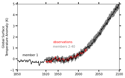
Figure will appear above when ready. Compare with Fig.2 of Kay et al. 2015 (doi:10.1175/BAMS-D-13-00255.1)

Compute linear trend for winter seasons

def linear_trend(da, dim="time"):
    da_chunk = da.chunk({dim: -1})
    trend = xr.apply_ufunc(
        calc_slope,
        da_chunk,
        vectorize=True,
        input_core_dims=[[dim]],
        output_core_dims=[[]],
        output_dtypes=[np.float],
        dask="parallelized",
    )
    return trend


def calc_slope(y):
    """ufunc to be used by linear_trend"""
    x = np.arange(len(y))

    # drop missing values (NaNs) from x and y
    finite_indexes = ~np.isnan(y)
    slope = np.nan if (np.sum(finite_indexes) < 2) else np.polyfit(x[finite_indexes], y[finite_indexes], 1)[0]
    return slope

Compute ensemble trends

t = xr.concat([t_20c, t_rcp], dim="time")
seasons = t.sel(time=slice("1979", "2012")).resample(time="QS-DEC").mean("time")
# Include only full seasons from 1979 and 2012
seasons = seasons.sel(time=slice("1979", "2012")).load()

winter_seasons = seasons.sel(
    time=seasons.time.where(seasons.time.dt.month == 12, drop=True)
)
winter_trends = linear_trend(
    winter_seasons.chunk({"lat": 20, "lon": 20, "time": -1})
).load() * len(winter_seasons.time)

# Compute ensemble mean from the first 30 members
winter_trends_mean = winter_trends.isel(member_id=range(30)).mean(dim='member_id')

# Make sure that we have 34 seasons
assert len(winter_seasons.time) == 34

Get Observations for Figure 4 (NASA GISS GisTemp)

# Observational time series data for comparison with ensemble average
# NASA GISS Surface Temperature Analysis, https://data.giss.nasa.gov/gistemp/
obsDataURL = "https://data.giss.nasa.gov/pub/gistemp/gistemp1200_GHCNv4_ERSSTv5.nc.gz"

# Download, unzip, and load file
import os
os.system("wget " + obsDataURL)

obsDataFileName = obsDataURL.split('/')[-1]
os.system("gunzip " + obsDataFileName)

obsDataFileName = obsDataFileName[:-3]
ds = xr.open_dataset(obsDataFileName).load()
ds

<xarray.Dataset>
Dimensions:      (lat: 90, lon: 180, nv: 2, time: 1687)
Coordinates:
  * lat          (lat) float32 -89.0 -87.0 -85.0 -83.0 ... 83.0 85.0 87.0 89.0
  * lon          (lon) float32 -179.0 -177.0 -175.0 -173.0 ... 175.0 177.0 179.0
  * time         (time) datetime64[ns] 1880-01-15 1880-02-15 ... 2020-07-15
Dimensions without coordinates: nv
Data variables:
    time_bnds    (time, nv) datetime64[ns] 1880-01-01 1880-02-01 ... 2020-08-01
    tempanomaly  (time, lat, lon) float32 nan nan nan nan ... 0.55 0.55 0.55
Attributes:
    title:        GISTEMP Surface Temperature Analysis
    institution:  NASA Goddard Institute for Space Studies
    source:       http://data.giss.nasa.gov/gistemp/
    Conventions:  CF-1.6
    history:      Created 2020-08-13 09:26:17 by SBBX_to_nc 2.0 - ILAND=1200,...

# Remap longitude range from [-180, 180] to [0, 360] for plotting purposes
ds = ds.assign_coords(lon=((ds.lon + 360) % 360)).sortby('lon')
ds

<xarray.Dataset>
Dimensions:      (lat: 90, lon: 180, nv: 2, time: 1687)
Coordinates:
  * lat          (lat) float32 -89.0 -87.0 -85.0 -83.0 ... 83.0 85.0 87.0 89.0
  * lon          (lon) float32 1.0 3.0 5.0 7.0 9.0 ... 353.0 355.0 357.0 359.0
  * time         (time) datetime64[ns] 1880-01-15 1880-02-15 ... 2020-07-15
Dimensions without coordinates: nv
Data variables:
    time_bnds    (time, nv) datetime64[ns] 1880-01-01 1880-02-01 ... 2020-08-01
    tempanomaly  (time, lat, lon) float32 nan nan nan nan ... 0.55 0.55 0.55
Attributes:
    title:        GISTEMP Surface Temperature Analysis
    institution:  NASA Goddard Institute for Space Studies
    source:       http://data.giss.nasa.gov/gistemp/
    Conventions:  CF-1.6
    history:      Created 2020-08-13 09:26:17 by SBBX_to_nc 2.0 - ILAND=1200,...

Compute observed trends

obs_seasons = ds.sel(time=slice("1979", "2012")).resample(time="QS-DEC").mean("time")
# Include only full seasons from 1979 through 2012
obs_seasons = obs_seasons.sel(time=slice("1979", "2012")).load()

# Compute observed winter trends
obs_winter_seasons = obs_seasons.sel(
    time=obs_seasons.time.where(obs_seasons.time.dt.month == 12, drop=True)
)
obs_winter_seasons

<xarray.Dataset>
Dimensions:      (lat: 90, lon: 180, time: 34)
Coordinates:
  * time         (time) datetime64[ns] 1979-12-01 1980-12-01 ... 2012-12-01
  * lon          (lon) float32 1.0 3.0 5.0 7.0 9.0 ... 353.0 355.0 357.0 359.0
  * lat          (lat) float32 -89.0 -87.0 -85.0 -83.0 ... 83.0 85.0 87.0 89.0
Data variables:
    tempanomaly  (time, lat, lon) float32 0.5333333 0.5333333 ... 7.47 7.47

obs_winter_trends = linear_trend(
    obs_winter_seasons.chunk({"lat": 20, "lon": 20, "time": -1})
).load() * len(obs_winter_seasons.time)
obs_winter_trends

<xarray.Dataset>
Dimensions:      (lat: 90, lon: 180)
Coordinates:
  * lon          (lon) float32 1.0 3.0 5.0 7.0 9.0 ... 353.0 355.0 357.0 359.0
  * lat          (lat) float32 -89.0 -87.0 -85.0 -83.0 ... 83.0 85.0 87.0 89.0
Data variables:
    tempanomaly  (lat, lon) float64 1.284 1.284 1.284 ... 5.672 5.672 5.672

Figure 4: Global maps of historical (1979 - 2012) boreal winter (DJF) surface air trends

import cmaps  # for NCL colormaps
import cartopy.crs as ccrs
import matplotlib.pyplot as plt

contour_levels = [-6, -5, -4, -3, -2, -1.5, -1, -0.5, 0, 0.5, 1, 1.5, 2, 3, 4, 5, 6]

color_map = cmaps.ncl_default

def make_map_plot(nplot_rows, nplot_cols, plot_index, data, plot_label):
    """ Create a single map subplot. """
    ax = plt.subplot(nplot_rows, nplot_cols, plot_index, projection = ccrs.Robinson(central_longitude = 180))
    cplot = plt.contourf(lons, lats, data,
                         levels = contour_levels,
                         cmap = color_map,
                         extend = 'both',
                         transform = ccrs.PlateCarree())
    ax.coastlines(color = 'grey')
    ax.text(0.01, 0.01, plot_label, fontSize = 14, transform = ax.transAxes)
    return cplot, ax

# Generate plot (may take a while as many individual maps are generated)
numPlotRows = 8
numPlotCols = 4
figWidth = 20
figHeight = 30

fig, axs = plt.subplots(numPlotRows, numPlotCols, figsize=(figWidth,figHeight))

lats = winter_trends.lat
lons = winter_trends.lon

# Create ensemble member plots
for ensemble_index in range(30):
    plot_data = winter_trends.isel(member_id = ensemble_index)
    plot_index = ensemble_index + 1
    plot_label = str(plot_index)
    plotRow = ensemble_index // numPlotCols
    plotCol = ensemble_index % numPlotCols
    # Retain axes objects for figure colorbar
    cplot, axs[plotRow, plotCol] = make_map_plot(numPlotRows, numPlotCols, plot_index, plot_data, plot_label)

# Create plots for the ensemble mean, observations, and a figure color bar.
cplot, axs[7,2] = make_map_plot(numPlotRows, numPlotCols, 31, winter_trends_mean, 'EM')

lats = obs_winter_trends.lat
lons = obs_winter_trends.lon
cplot, axs[7,3] = make_map_plot(numPlotRows, numPlotCols, 32, obs_winter_trends.tempanomaly, 'OBS')

cbar = fig.colorbar(cplot, ax=axs, orientation='horizontal', shrink = 0.7, pad = 0.02)
cbar.ax.set_title('1979-2012 DJF surface air temperature trends (K/34 years)', fontSize = 16)
cbar.set_ticks(contour_levels)
cbar.set_ticklabels(contour_levels)

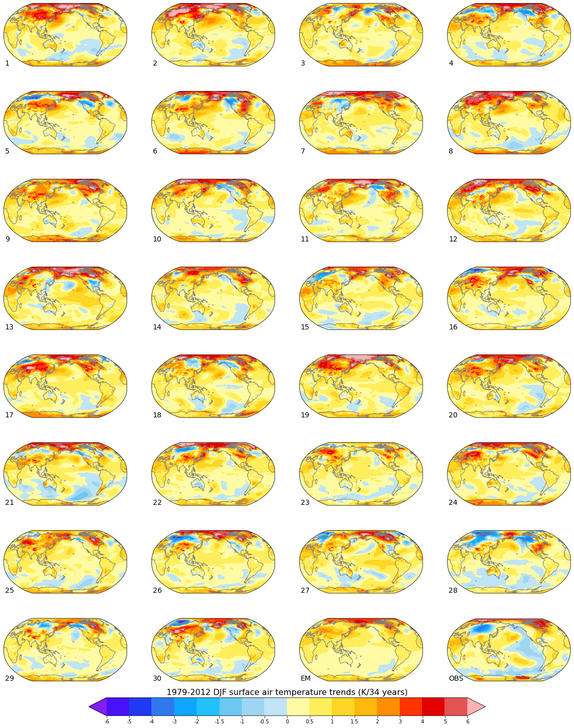
Figure will appear above when ready. Compare with Fig. 4 of Kay et al. 2015 (doi:10.1175/BAMS-D-13-00255.1).

# Gracefully destroy/close our cluster
client.close()
cluster.close()