Bias Correction¶

This notebook demonstrates z-score bias correction in 4 steps:

Look at zonal wind data
Filtering the data to the extent of Colorado
Aligning the datasets in time
A z-score bias correction method

Set up Workspace¶

Import all necessary modules and name the variable we will be looking at (zonal wind speed, uas).

[1]:

import xarray as xr
import numpy as np
import matplotlib.pyplot as plt
from scipy import interpolate, stats
import xesmf as xe
from datetime import datetime, timedelta
from ngallery_utils import DATASETS

%matplotlib inline

var = 'uas'

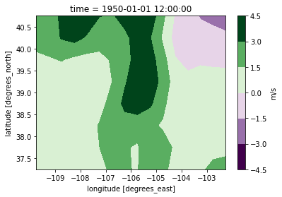
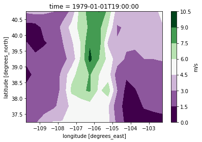
1. Look at Data¶

We have 3 datasets for this correction: a historical model, a future rcp85 model, and measurements.

Ultimately, the historical model will be compared to the measurements to predict an adjustment to the future rcp85 model to be more like future measurements.

[2]:

hist_file = DATASETS.fetch("uas.hist.CanESM2.CRCM5-UQAM.day.NAM-44i.raw.Colorado.nc")
rcp85_file = DATASETS.fetch("uas.rcp85.CanESM2.CRCM5-UQAM.day.NAM-44i.raw.Colorado.nc")
meas_file = DATASETS.fetch("uas.gridMET.NAM-44i.Colorado.nc")

Downloading file 'uas.hist.CanESM2.CRCM5-UQAM.day.NAM-44i.raw.Colorado.nc' from 'ftp://ftp.cgd.ucar.edu/archive/aletheia-data/tutorial-data/uas.hist.CanESM2.CRCM5-UQAM.day.NAM-44i.raw.Colorado.nc' to '/home/jovyan/aletheia-data/tutorial-data'.
Downloading file 'uas.rcp85.CanESM2.CRCM5-UQAM.day.NAM-44i.raw.Colorado.nc' from 'ftp://ftp.cgd.ucar.edu/archive/aletheia-data/tutorial-data/uas.rcp85.CanESM2.CRCM5-UQAM.day.NAM-44i.raw.Colorado.nc' to '/home/jovyan/aletheia-data/tutorial-data'.
Downloading file 'uas.gridMET.NAM-44i.Colorado.nc' from 'ftp://ftp.cgd.ucar.edu/archive/aletheia-data/tutorial-data/uas.gridMET.NAM-44i.Colorado.nc' to '/home/jovyan/aletheia-data/tutorial-data'.

# Or if not on Cheyenne hist_file = DATASERTS.fetch("/uas.hist.CanESM2.CRCM5-UQAM.day.NAM-44i.raw.Colorado.nc") rcp85_file = DATASERTS.fetch("/uas.rcp85.CanESM2.CRCM5-UQAM.day.NAM-44i.raw.Colorado.nc") meas_file = DATASETS.fetch("uas.gridMET.NAM-44i.Colorado.nc")

[3]:

ds_hist = xr.open_dataset(hist_file)
ds_hist

[4]:

ds_hist[var].isel(time=0).plot.contourf(x="lon", y="lat", cmap="PRGn", cbar_kwargs={"label": "m/s"})

[4]:

<matplotlib.contour.QuadContourSet at 0x7fc0757430a0>

../../../../../../_images/repos_NCAR_notebook-gallery_notebooks_Run-Anywhere_Bias-Correction_bias_correction_7_1.png

[5]:

ds_rcp85 = xr.open_dataset(rcp85_file)
ds_rcp85

[6]:

ds_rcp85[var].isel(time=0).plot.contourf(x="lon", y="lat", cmap="PRGn", cbar_kwargs={"label": "m/s"})

[6]:

<matplotlib.contour.QuadContourSet at 0x7fc074bb0b20>

../../../../../../_images/repos_NCAR_notebook-gallery_notebooks_Run-Anywhere_Bias-Correction_bias_correction_9_1.png

[7]:

ds_meas = xr.open_dataset(meas_file)
ds_meas

[8]:

ds_meas[var].isel(time=0).plot.contourf(x="lon", y="lat", cmap="PRGn", cbar_kwargs={"label": "m/s"})

[8]:

<matplotlib.contour.QuadContourSet at 0x7fc074e57520>

../../../../../../_images/repos_NCAR_notebook-gallery_notebooks_Run-Anywhere_Bias-Correction_bias_correction_11_1.png

2. Filter Data¶

We limit the extent of our data to the state of Colorado simply to speed up our calculations in this example.

[9]:

wesn = [-110, -108, 39.5, 41.5]
ds_meas_flt = ds_meas.sel(lon = slice(wesn[0], wesn[1]), lat = slice(wesn[2], wesn[3]))
ds_hist_flt = ds_hist.sel(lon = slice(wesn[0], wesn[1]), lat = slice(wesn[2], wesn[3]))
ds_rcp85_flt = ds_rcp85.sel(lon = slice(wesn[0], wesn[1]), lat = slice(wesn[2], wesn[3]))

3. Align Time¶

Our two modeled datasets do not have leap years, where our measured dataset does.

There are several methods of dealing with leap years that are better for different types of data. For data that is continuous, such as wind speed, we can simply drop all December 31st from leap years (any time there is a 366th day to the year we drop day #366). This method would not be ideal for discontinous data such as precipitation.

[10]:

ds_meas_noleap = ds_meas_flt.sel(time=~((ds_meas_flt.time.dt.dayofyear == 366) ))

[11]:

def _cfnoleap_to_datetime(da):
    datetimeindex = da.indexes['time'].to_datetimeindex()
    ds = da#.to_dataset()
    ds['time_dt']= ('time', datetimeindex)
    ds = ds.swap_dims({'time': 'time_dt'})
    assert len(da.time) == len(ds.time_dt)
    return ds

ds_hist_dt = _cfnoleap_to_datetime(ds_hist_flt)
ds_rcp85_dt = _cfnoleap_to_datetime(ds_rcp85_flt)

<ipython-input-1-d460699fd441>:2: RuntimeWarning: Converting a CFTimeIndex with dates from a non-standard calendar, 'noleap', to a pandas.DatetimeIndex, which uses dates from the standard calendar.  This may lead to subtle errors in operations that depend on the length of time between dates.
  datetimeindex = da.indexes['time'].to_datetimeindex()

We also regroup our models so that the dates of the historical model line up with our historical measurements.

[12]:

def _regroup_models_bytime(ds_meas, ds_hist_dt, ds_rcp_dt):
    t0_meas = ds_meas.time[0]
    tn_meas = ds_meas.time[-1]
    t0_fut = tn_meas.values + np.timedelta64(1, 'D')

    ds_past = ds_hist_dt.sel(time_dt = slice(t0_meas, tn_meas))
    ds_past = ds_past.swap_dims({'time_dt':'time'})

    ds_fut_pt1 = ds_hist_dt.sel(time_dt = slice(t0_fut,None))
    ds_fut = xr.concat([ds_fut_pt1[var], ds_rcp_dt[var]], 'time_dt')
    ds_fut = ds_fut.swap_dims({'time_dt':'time'})
    return ds_past, ds_fut

ds_past, ds_fut = _regroup_models_bytime(ds_meas_noleap, ds_hist_dt, ds_rcp85_dt)

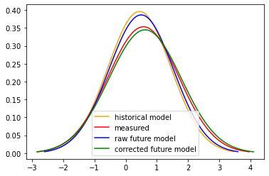
4. Z-score Bias Correction¶

Z-Score bias correction is a good technique for target variables with Gaussian probability distributions, such as zonal wind speed.

In essence the technique:

Finds the mean

\[\overline{x} = \sum_{i=0}^N \frac{x_i}{N}\]

and standard deviation

\[\sigma = \sqrt{\frac{\sum_{i=0}^N |x_i - \overline{x}|^2}{N-1}}\]

of target (measured) data and training (historical modeled) data.
Compares the difference between the statistical values to produce a shift

\[shift = \overline{x_{target}} - \overline{x_{training}}\]

and scale parameter

\[scale = \sigma_{target} \div \sigma_{training}\]
Applies these paramaters to the future model data to be corrected to get a new mean

\[\overline{x_{corrected}} = \overline{x_{future}} + shift\]

and new standard deviation

\[\sigma_{corrected} = \sigma_{future} \times scale\]
Calculates the corrected values

\[x_{corrected_{i}} = z_i \times \sigma_{corrected} + \overline{x_{corrected}}\]

from the future model’s z-score values

\[z_i = \frac{x_i-\overline{x}}{\sigma}\]

In practice, if the wind was on average 3 m/s faster on the first of July in the models compared to the measurements, we would adjust the modeled data for all July 1sts in the future modeled dataset to be 3 m/s faster. And similarly for scaling the standard deviation

Bias correction methods other than zscore include:

scale (for wind speed, wave flux in air)
log (for precipitation)
range (relative humidity)
seth mcginnes’s kddm (for any bimodal distributions)

[13]:

def _reshape(ds, window_width):
    split = lambda g: (g.rename({'time': 'day'})
                       .assign_coords(day=g.time.dt.dayofyear.values))
    ds2 = ds.groupby('time.year').apply(split)

    early_Jans = ds2.isel(day = slice(None,window_width//2))
    late_Decs = ds2.isel(day = slice(-window_width//2,None))

    ds3 = xr.concat([late_Decs,ds2,early_Jans],dim='day')
    return ds3

def _calc_stats(ds, window_width):
    ds_rsh = _reshape(ds, window_width)

    ds_rolled = ds_rsh.rolling(day=window_width, center=True).construct('win_day')

    n = window_width//2+1
    ds_mean = ds_rolled.mean(dim=['year','win_day']).isel(day=slice(n,-n))
    ds_std = ds_rolled.std(dim=['year','win_day']).isel(day=slice(n,-n))

    ds_avyear = ds_rsh.mean(dim=['year','day'])
    ds_zscore = ((ds_avyear - ds_mean) / ds_std)
    return ds_mean, ds_std, ds_zscore

window_width=31
meas_mean, meas_std, meas_zscore = _calc_stats(ds_meas_noleap, window_width)
hist_mean, hist_std, hist_zscore = _calc_stats(ds_past, window_width)

[14]:

def _get_params(meas_mean, meas_std, past_mean, past_std):
    shift = meas_mean - past_mean
    scale = meas_std / past_std
    return shift, scale

shift, scale = _get_params(meas_mean, meas_std, hist_mean, hist_std)

[15]:

def _calc_fut_stats(ds_fut, window_width):
    ds_rolled = ds_fut.rolling(time=window_width, center=True).construct('win_day')

    ds_mean = ds_rolled.mean(dim=['win_day'])
    ds_std = ds_rolled.std(dim=['win_day'])

    ds_avyear = ds_fut.mean(dim=['time'])
    ds_zscore = ((ds_avyear - ds_mean) / ds_std)
    return ds_mean, ds_std, ds_zscore

fut_mean, fut_std, fut_zscore = _calc_fut_stats(ds_fut, window_width)

[16]:

fut_mean_bc = fut_mean + shift.uas
fut_std_bc = fut_std * scale

[17]:

fut_corrected = (fut_zscore * fut_std_bc) + fut_mean_bc

Visualize the Correction¶

[18]:

def gaus(mean, std, doy):
    a = mean.sel(day=doy)
    mu = a.isel(lon = 0, lat = 0)

    b =std.sel(day=doy)
    sigma = b.isel(lon = 0, lat = 0)

    x = np.linspace(mu - 3*sigma, mu + 3*sigma, 100)
    y = stats.norm.pdf(x, mu, sigma)
    return x, y

[19]:

fut_typ_mean, fut_typ_std, fut_typ_zscore = _calc_stats(ds_fut, window_width)
fut_typ_mean_bc = fut_typ_mean + shift
fut_typ_std_bc = fut_typ_std * scale

doy=20
plt.figure()
x,y = gaus(hist_mean[var], hist_std[var], doy)
plt.plot(x, y, 'orange', label = 'historical model')
x,y = gaus(meas_mean[var], meas_std[var], doy)
plt.plot(x, y, 'red', label = 'measured')
x,y = gaus(fut_typ_mean, fut_typ_std, doy)
plt.plot(x, y, 'blue', label = 'raw future model')
x,y = gaus(fut_typ_mean_bc[var], fut_typ_std_bc[var], doy)
plt.plot(x, y, 'green', label = 'corrected future model')
plt.legend()

[19]:

<matplotlib.legend.Legend at 0x7fc074acd220>

../../../../../../_images/repos_NCAR_notebook-gallery_notebooks_Run-Anywhere_Bias-Correction_bias_correction_27_1.png