Along Track Altimetry Analysis¶

[1]:

import fsspec
import xarray as xr
import numpy as np
import hvplot
import hvplot.dask
import hvplot.pandas
import hvplot.xarray

Load Data¶

The analysis ready along-track altimetry data were prepared by CNES. They are catalogged in the Pangeo Cloud Data Catalog here: https://catalog.pangeo.io/browse/master/ocean/altimetry/

We work with Jason 3.

[2]:

from intake import open_catalog
cat = open_catalog("https://raw.githubusercontent.com/pangeo-data/pangeo-datastore/master/intake-catalogs/ocean/altimetry.yaml")
print(list(cat))
ds = cat['j3'].to_dask()
ds

['al', 'alg', 'c2', 'e1', 'e1g', 'e2', 'en', 'enn', 'g2', 'h2', 'j1', 'j1g', 'j1n', 'j2', 'j2g', 'j2n', 'j3', 's3a', 's3b', 'tp', 'tpn']

[2]:

<xarray.Dataset>
Dimensions:         (time: 53154815)
Coordinates:
    latitude        (time) float64 dask.array<chunksize=(53154815,), meta=np.ndarray>
    longitude       (time) float64 dask.array<chunksize=(53154815,), meta=np.ndarray>
  * time            (time) datetime64[ns] 2016-05-26T14:14:03.917554 ... 2019...
Data variables:
    cycle           (time) int16 dask.array<chunksize=(53154815,), meta=np.ndarray>
    dac             (time) float64 dask.array<chunksize=(53154815,), meta=np.ndarray>
    lwe             (time) float64 dask.array<chunksize=(53154815,), meta=np.ndarray>
    mdt             (time) float64 dask.array<chunksize=(53154815,), meta=np.ndarray>
    ocean_tide      (time) float64 dask.array<chunksize=(53154815,), meta=np.ndarray>
    sla_filtered    (time) float64 dask.array<chunksize=(53154815,), meta=np.ndarray>
    sla_unfiltered  (time) float64 dask.array<chunksize=(53154815,), meta=np.ndarray>
    track           (time) int16 dask.array<chunksize=(53154815,), meta=np.ndarray>
Attributes: (12/24)
    Conventions:               CF-1.6
    Metadata_Conventions:      Unidata Dataset Discovery v1.0
    cdm_data_type:             Swath
    comment:                   Sea surface height measured by altimeters refe...
    contact:                   servicedesk.cmems@mercator-ocean.eu
    creator_email:             servicedesk.cmems@mercator-ocean.eu
    ...                        ...
    software_version:          6.2_DUACS_DT2018_baseline
    source:                    Jason-3 measurements
    ssalto_duacs_comment:      The reference mission used for the altimeter i...
    standard_name_vocabulary:  NetCDF Climate and Forecast (CF) Metadata Conv...
    summary:                   SSALTO/DUACS Delayed-Time Level-3 sea surface ...
    title:                     DT Jason-3 Global Ocean Along track SSALTO/DUA...

xarray.Dataset

Dimensions:
- time: 53154815

Coordinates: (3)

latitude

(time)

float64

dask.array<chunksize=(53154815,), meta=np.ndarray>

long_name :: Latitude of measurement
standard_name :: latitude
units :: degrees_north

	Array	Chunk
Bytes	405.54 MiB	405.54 MiB
Shape	(53154815,)	(53154815,)
Count	2 Tasks	1 Chunks
Type	float64	numpy.ndarray

longitude

(time)

float64

dask.array<chunksize=(53154815,), meta=np.ndarray>

long_name :: Longitude of measurement
standard_name :: longitude
units :: degrees_east

	Array	Chunk
Bytes	405.54 MiB	405.54 MiB
Shape	(53154815,)	(53154815,)
Count	2 Tasks	1 Chunks
Type	float64	numpy.ndarray

time

(time)

datetime64[ns]

2016-05-26T14:14:03.917554 ... 2...

axis :: T
long_name :: Time of measurement
standard_name :: time

array(['2016-05-26T14:14:03.917554000', '2016-05-26T14:14:04.996134000',
       '2016-05-26T14:14:06.074715000', ..., '2019-05-13T23:58:11.995103000',
       '2019-05-13T23:58:13.073683000', '2019-05-13T23:58:14.152263000'],
      dtype='datetime64[ns]')

Data variables: (8)

cycle

(time)

int16

dask.array<chunksize=(53154815,), meta=np.ndarray>

long_name :: Cycle the measurement belongs to
units :: 1

	Array	Chunk
Bytes	101.38 MiB	101.38 MiB
Shape	(53154815,)	(53154815,)
Count	2 Tasks	1 Chunks
Type	int16	numpy.ndarray

dac

(time)

float64

dask.array<chunksize=(53154815,), meta=np.ndarray>

comment :: The sla in this file is already corrected for the dac; the uncorrected sla can be computed as follows: [uncorrected sla]=[sla from product]+[dac]; see the product user manual for details
long_name :: Dynamic Atmospheric Correction
units :: m

	Array	Chunk
Bytes	405.54 MiB	405.54 MiB
Shape	(53154815,)	(53154815,)
Count	2 Tasks	1 Chunks
Type	float64	numpy.ndarray

lwe

(time)

float64

dask.array<chunksize=(53154815,), meta=np.ndarray>

comment :: The sla in this file is already corrected for the lwe; the uncorrected sla can be computed as follows: [uncorrected sla]=[sla from product]-[lwe]; see the product user manual for details
long_name :: Long wavelength error
units :: m

	Array	Chunk
Bytes	405.54 MiB	405.54 MiB
Shape	(53154815,)	(53154815,)
Count	2 Tasks	1 Chunks
Type	float64	numpy.ndarray

mdt

(time)

float64

dask.array<chunksize=(53154815,), meta=np.ndarray>

comment :: The mean dynamic topography is the sea surface height above geoid; it is used to compute the absolute dynamic tyopography adt=sla+mdt
long_name :: Mean dynamic topography
standard_name :: sea_surface_height_above_geoid
units :: m

	Array	Chunk
Bytes	405.54 MiB	405.54 MiB
Shape	(53154815,)	(53154815,)
Count	2 Tasks	1 Chunks
Type	float64	numpy.ndarray

ocean_tide

(time)

float64

dask.array<chunksize=(53154815,), meta=np.ndarray>

comment :: The sla in this file is already corrected for the ocean_tide; the uncorrected sla can be computed as follows: [uncorrected sla]=[sla from product]+[ocean_tide]; see the product user manual for details
long_name :: Ocean tide model
units :: m

	Array	Chunk
Bytes	405.54 MiB	405.54 MiB
Shape	(53154815,)	(53154815,)
Count	2 Tasks	1 Chunks
Type	float64	numpy.ndarray

sla_filtered

(time)

float64

dask.array<chunksize=(53154815,), meta=np.ndarray>

comment :: The sea level anomaly is the sea surface height above mean sea surface height; the uncorrected sla can be computed as follows: [uncorrected sla]=[sla from product]+[dac]+[ocean_tide]-[lwe]; see the product user manual for details
long_name :: Sea level anomaly filtered not-subsampled with dac, ocean_tide and lwe correction applied
standard_name :: sea_surface_height_above_sea_level
units :: m

	Array	Chunk
Bytes	405.54 MiB	405.54 MiB
Shape	(53154815,)	(53154815,)
Count	2 Tasks	1 Chunks
Type	float64	numpy.ndarray

sla_unfiltered

(time)

float64

dask.array<chunksize=(53154815,), meta=np.ndarray>

comment :: The sea level anomaly is the sea surface height above mean sea surface height; the uncorrected sla can be computed as follows: [uncorrected sla]=[sla from product]+[dac]+[ocean_tide]-[lwe]; see the product user manual for details
long_name :: Sea level anomaly not-filtered not-subsampled with dac, ocean_tide and lwe correction applied
standard_name :: sea_surface_height_above_sea_level
units :: m

	Array	Chunk
Bytes	405.54 MiB	405.54 MiB
Shape	(53154815,)	(53154815,)
Count	2 Tasks	1 Chunks
Type	float64	numpy.ndarray

track

(time)

int16

dask.array<chunksize=(53154815,), meta=np.ndarray>

long_name :: Track in cycle the measurement belongs to
units :: 1

	Array	Chunk
Bytes	101.38 MiB	101.38 MiB
Shape	(53154815,)	(53154815,)
Count	2 Tasks	1 Chunks
Type	int16	numpy.ndarray

Attributes: (24)
Conventions :
CF-1.6
Metadata_Conventions :
Unidata Dataset Discovery v1.0
cdm_data_type :
Swath
comment :
Sea surface height measured by altimeters referenced to the [1993, 2012] period; with additional corrections; the proposed sla is already corrected for dac, ocean_tide and lwe; [uncorrected sla]=[sla from product]+[dac]+[ocean_tide]-[lwe]
contact :
servicedesk.cmems@mercator-ocean.eu
creator_email :
servicedesk.cmems@mercator-ocean.eu
creator_name :
CMEMS - Sea Level Thematic Assembly Center
creator_url :
http://marine.copernicus.eu
history :
2019-02-20T12:45:46Z: Creation
institution :
CLS, CNES, EUMETSAT
keywords :
Oceans > Ocean Topography > Sea Surface Height
keywords_vocabulary :
NetCDF COARDS Climate and Forecast Standard Names
license :
http://marine.copernicus.eu/web/27-service-commitments-and-licence.php
platform :
Jason-3
processing_level :
L3
product_version :
2019
project :
EUMETSAT Jason-3 L2P/L3 Marine Altimetry Service
references :
http://marine.copernicus.eu
software_version :
6.2_DUACS_DT2018_baseline
source :
Jason-3 measurements
ssalto_duacs_comment :
The reference mission used for the altimeter inter-calibration processing is Topex/Poseidon between 1993-01-01 and 2002-04-23, Jason-1 between 2002-04-24 and 2008-10-18, OSTM/Jason-2 between 2008-10-19 and 2016-06-25, Jason-3 since 2016-06-25.
standard_name_vocabulary :
NetCDF Climate and Forecast (CF) Metadata Convention Standard Name Table v37
summary :
SSALTO/DUACS Delayed-Time Level-3 sea surface height measured by Jason-3 altimetry observations over Global Ocean.
title :
DT Jason-3 Global Ocean Along track SSALTO/DUACS Sea Surface Height L3 product

Load somed data into memory:

[3]:

ds_ll = ds[['latitude', 'longitude', 'sla_filtered']].reset_coords().astype('f4').load()
ds_ll

Convert to pandas dataframe:

[4]:

df = ds_ll.to_dataframe()
df

[4]:

	latitude	longitude	sla_filtered
time
2016-05-26 14:14:03.917554	-66.147430	17.224194	0.026
2016-05-26 14:14:04.996134	-66.147163	17.361219	0.028
2016-05-26 14:14:06.074715	-66.146767	17.498243	0.030
2016-05-26 14:14:07.153295	-66.146240	17.635262	0.031
2016-05-26 14:14:08.231875	-66.145592	17.772272	0.032
...	...	...	...
2019-05-13 23:58:09.837942	66.142929	335.137817	0.120
2019-05-13 23:58:10.916522	66.143593	335.274872	0.125
2019-05-13 23:58:11.995103	66.144127	335.411926	0.129
2019-05-13 23:58:13.073683	66.144539	335.548981	0.134
2019-05-13 23:58:14.152263	66.144814	335.686066	0.138

53154815 rows × 3 columns

Visualize with hvplot¶

[5]:

df.hvplot.scatter(x='longitude', y='latitude', datashade=True, )

[5]:

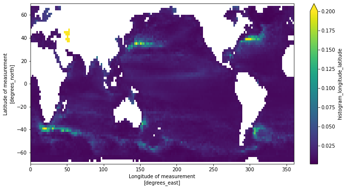
Bin using xhistogram¶

https://xhistogram.readthedocs.io/

[6]:

from xhistogram.xarray import histogram

lon_bins = np.arange(0, 361, 2)
lat_bins = np.arange(-70, 71, 2)

# helps with memory management
ds_ll_chunked = ds_ll.chunk({'time': '5MB'})

sla_variance = histogram(ds_ll_chunked.longitude, ds_ll_chunked.latitude,
                         bins=[lon_bins, lat_bins],
                         weights=ds_ll_chunked.sla_filtered.fillna(0.)**2)

norm = histogram(ds_ll_chunked.longitude, ds_ll_chunked.latitude,
                         bins=[lon_bins, lat_bins])


# let's get at least 200 points in a box for it to be unmasked
thresh = 200
sla_variance = sla_variance / norm.where(norm > thresh)
sla_variance

[6]:

<xarray.DataArray 'histogram_longitude_latitude' (longitude_bin: 180, latitude_bin: 70)>
dask.array<truediv, shape=(180, 70), dtype=float64, chunksize=(180, 70), chunktype=numpy.ndarray>
Coordinates:
  * longitude_bin  (longitude_bin) float64 1.0 3.0 5.0 7.0 ... 355.0 357.0 359.0
  * latitude_bin   (latitude_bin) float64 -69.0 -67.0 -65.0 ... 65.0 67.0 69.0

xarray.DataArray

'histogram_longitude_latitude'

longitude_bin: 180
latitude_bin: 70

dask.array<chunksize=(180, 70), meta=np.ndarray>

	Array	Chunk
Bytes	98.44 kiB	98.44 kiB
Shape	(180, 70)	(180, 70)
Count	507 Tasks	1 Chunks
Type	float64	numpy.ndarray

Coordinates: (2)

longitude_bin

(longitude_bin)

float64

1.0 3.0 5.0 ... 355.0 357.0 359.0

long_name :: Longitude of measurement
standard_name :: longitude
units :: degrees_east

array([  1.,   3.,   5.,   7.,   9.,  11.,  13.,  15.,  17.,  19.,  21.,  23.,
        25.,  27.,  29.,  31.,  33.,  35.,  37.,  39.,  41.,  43.,  45.,  47.,
        49.,  51.,  53.,  55.,  57.,  59.,  61.,  63.,  65.,  67.,  69.,  71.,
        73.,  75.,  77.,  79.,  81.,  83.,  85.,  87.,  89.,  91.,  93.,  95.,
        97.,  99., 101., 103., 105., 107., 109., 111., 113., 115., 117., 119.,
       121., 123., 125., 127., 129., 131., 133., 135., 137., 139., 141., 143.,
       145., 147., 149., 151., 153., 155., 157., 159., 161., 163., 165., 167.,
       169., 171., 173., 175., 177., 179., 181., 183., 185., 187., 189., 191.,
       193., 195., 197., 199., 201., 203., 205., 207., 209., 211., 213., 215.,
       217., 219., 221., 223., 225., 227., 229., 231., 233., 235., 237., 239.,
       241., 243., 245., 247., 249., 251., 253., 255., 257., 259., 261., 263.,
       265., 267., 269., 271., 273., 275., 277., 279., 281., 283., 285., 287.,
       289., 291., 293., 295., 297., 299., 301., 303., 305., 307., 309., 311.,
       313., 315., 317., 319., 321., 323., 325., 327., 329., 331., 333., 335.,
       337., 339., 341., 343., 345., 347., 349., 351., 353., 355., 357., 359.])

latitude_bin

(latitude_bin)

float64

-69.0 -67.0 -65.0 ... 67.0 69.0

long_name :: Latitude of measurement
standard_name :: latitude
units :: degrees_north

array([-69., -67., -65., -63., -61., -59., -57., -55., -53., -51., -49., -47.,
       -45., -43., -41., -39., -37., -35., -33., -31., -29., -27., -25., -23.,
       -21., -19., -17., -15., -13., -11.,  -9.,  -7.,  -5.,  -3.,  -1.,   1.,
         3.,   5.,   7.,   9.,  11.,  13.,  15.,  17.,  19.,  21.,  23.,  25.,
        27.,  29.,  31.,  33.,  35.,  37.,  39.,  41.,  43.,  45.,  47.,  49.,
        51.,  53.,  55.,  57.,  59.,  61.,  63.,  65.,  67.,  69.])

Attributes: (0)

[7]:

sla_variance.load()

[7]:

<xarray.DataArray 'histogram_longitude_latitude' (longitude_bin: 180, latitude_bin: 70)>
array([[       nan, 0.00620336, 0.00644503, ..., 0.01241829, 0.01244138,
               nan],
       [       nan, 0.00597437, 0.00593017, ..., 0.01349369, 0.01050862,
               nan],
       [       nan, 0.00590221, 0.00598762, ..., 0.01173668, 0.00958628,
               nan],
       ...,
       [       nan, 0.00657664, 0.00591848, ..., 0.00922974, 0.00990859,
               nan],
       [       nan, 0.00629435, 0.00607831, ..., 0.01104878, 0.0128521 ,
               nan],
       [       nan, 0.00647509, 0.00636302, ..., 0.01209499, 0.01273962,
               nan]])
Coordinates:
  * longitude_bin  (longitude_bin) float64 1.0 3.0 5.0 7.0 ... 355.0 357.0 359.0
  * latitude_bin   (latitude_bin) float64 -69.0 -67.0 -65.0 ... 65.0 67.0 69.0

xarray.DataArray

'histogram_longitude_latitude'

longitude_bin: 180
latitude_bin: 70

nan 0.006203 0.006445 0.007156 ... 0.01286 0.01209 0.01274 nan

array([[       nan, 0.00620336, 0.00644503, ..., 0.01241829, 0.01244138,
               nan],
       [       nan, 0.00597437, 0.00593017, ..., 0.01349369, 0.01050862,
               nan],
       [       nan, 0.00590221, 0.00598762, ..., 0.01173668, 0.00958628,
               nan],
       ...,
       [       nan, 0.00657664, 0.00591848, ..., 0.00922974, 0.00990859,
               nan],
       [       nan, 0.00629435, 0.00607831, ..., 0.01104878, 0.0128521 ,
               nan],
       [       nan, 0.00647509, 0.00636302, ..., 0.01209499, 0.01273962,
               nan]])

Coordinates: (2)

longitude_bin

(longitude_bin)

float64

1.0 3.0 5.0 ... 355.0 357.0 359.0

long_name :: Longitude of measurement
standard_name :: longitude
units :: degrees_east

array([  1.,   3.,   5.,   7.,   9.,  11.,  13.,  15.,  17.,  19.,  21.,  23.,
        25.,  27.,  29.,  31.,  33.,  35.,  37.,  39.,  41.,  43.,  45.,  47.,
        49.,  51.,  53.,  55.,  57.,  59.,  61.,  63.,  65.,  67.,  69.,  71.,
        73.,  75.,  77.,  79.,  81.,  83.,  85.,  87.,  89.,  91.,  93.,  95.,
        97.,  99., 101., 103., 105., 107., 109., 111., 113., 115., 117., 119.,
       121., 123., 125., 127., 129., 131., 133., 135., 137., 139., 141., 143.,
       145., 147., 149., 151., 153., 155., 157., 159., 161., 163., 165., 167.,
       169., 171., 173., 175., 177., 179., 181., 183., 185., 187., 189., 191.,
       193., 195., 197., 199., 201., 203., 205., 207., 209., 211., 213., 215.,
       217., 219., 221., 223., 225., 227., 229., 231., 233., 235., 237., 239.,
       241., 243., 245., 247., 249., 251., 253., 255., 257., 259., 261., 263.,
       265., 267., 269., 271., 273., 275., 277., 279., 281., 283., 285., 287.,
       289., 291., 293., 295., 297., 299., 301., 303., 305., 307., 309., 311.,
       313., 315., 317., 319., 321., 323., 325., 327., 329., 331., 333., 335.,
       337., 339., 341., 343., 345., 347., 349., 351., 353., 355., 357., 359.])

latitude_bin

(latitude_bin)

float64

-69.0 -67.0 -65.0 ... 67.0 69.0

long_name :: Latitude of measurement
standard_name :: latitude
units :: degrees_north

array([-69., -67., -65., -63., -61., -59., -57., -55., -53., -51., -49., -47.,
       -45., -43., -41., -39., -37., -35., -33., -31., -29., -27., -25., -23.,
       -21., -19., -17., -15., -13., -11.,  -9.,  -7.,  -5.,  -3.,  -1.,   1.,
         3.,   5.,   7.,   9.,  11.,  13.,  15.,  17.,  19.,  21.,  23.,  25.,
        27.,  29.,  31.,  33.,  35.,  37.,  39.,  41.,  43.,  45.,  47.,  49.,
        51.,  53.,  55.,  57.,  59.,  61.,  63.,  65.,  67.,  69.])

Attributes: (0)

[8]:

sla_variance.plot(x='longitude_bin', figsize=(12, 6), vmax=0.2)

[8]:

<matplotlib.collections.QuadMesh at 0x7f78955daf10>

../../../_images/repos_pangeo-gallery_physical-oceanography_02_along_track_13_1.png

[ ]: