
Fancier example of transform
So you have thought of maybe interpolating your ocean data to a different depth grid or - the classic - interpolating onto temperature/density layers with `xgcm.Grid.transform <https://xgcm.readthedocs.io/en/latest/transform.html#>`__. But these are only a few options.
Lets go through a bit different example here: Transforming the data to a modified depth coordinate system based on a time variable diagnostic, like the mixed layer depth.
This can also be applied to other diagnostics, like e.g. the euphotic zone depth or others
First lets get some processing resources…
[1]:
from dask_gateway import GatewayCluster
from distributed import Client

cluster = GatewayCluster()
cluster.scale(6)
client = Client(cluster)
client
[1]:
Client
|
Cluster
|
Then load GFDL’s high resolution climate model CM2.6 as an example:
[2]:
from intake import open_catalog
import matplotlib.pyplot as plt
import xarray as xr
[3]:
cat = open_catalog("https://raw.githubusercontent.com/pangeo-data/pangeo-datastore/master/intake-catalogs/ocean/GFDL_CM2.6.yaml")
ds  = cat["GFDL_CM2_6_control_ocean"].to_dask()
ds
/srv/conda/envs/notebook/lib/python3.8/site-packages/xarray/coding/times.py:427: SerializationWarning: Unable to decode time axis into full numpy.datetime64 objects, continuing using cftime.datetime objects instead, reason: dates out of range
  dtype = _decode_cf_datetime_dtype(data, units, calendar, self.use_cftime)
[3]:
<xarray.Dataset>
Dimensions:            (nv: 2, st_edges_ocean: 51, st_ocean: 50, sw_edges_ocean: 51, sw_ocean: 50, time: 240, xt_ocean: 3600, xu_ocean: 3600, yt_ocean: 2700, yu_ocean: 2700)
Coordinates:
    geolat_c           (yu_ocean, xu_ocean) float32 dask.array<chunksize=(2700, 3600), meta=np.ndarray>
    geolat_t           (yt_ocean, xt_ocean) float32 dask.array<chunksize=(2700, 3600), meta=np.ndarray>
    geolon_c           (yu_ocean, xu_ocean) float32 dask.array<chunksize=(2700, 3600), meta=np.ndarray>
    geolon_t           (yt_ocean, xt_ocean) float32 dask.array<chunksize=(2700, 3600), meta=np.ndarray>
  * nv                 (nv) float64 1.0 2.0
  * st_edges_ocean     (st_edges_ocean) float64 0.0 10.07 ... 5.29e+03 5.5e+03
  * st_ocean           (st_ocean) float64 5.034 15.1 ... 5.185e+03 5.395e+03
  * sw_edges_ocean     (sw_edges_ocean) float64 5.034 15.1 ... 5.395e+03 5.5e+03
  * sw_ocean           (sw_ocean) float64 10.07 20.16 30.29 ... 5.29e+03 5.5e+03
  * time               (time) object 0181-01-16 12:00:00 ... 0200-12-16 12:00:00
  * xt_ocean           (xt_ocean) float64 -279.9 -279.8 -279.7 ... 79.85 79.95
  * xu_ocean           (xu_ocean) float64 -279.9 -279.8 -279.7 ... 79.9 80.0
  * yt_ocean           (yt_ocean) float64 -81.11 -81.07 -81.02 ... 89.94 89.98
  * yu_ocean           (yu_ocean) float64 -81.09 -81.05 -81.0 ... 89.96 90.0
Data variables:
    average_DT         (time) timedelta64[ns] dask.array<chunksize=(12,), meta=np.ndarray>
    average_T1         (time) object dask.array<chunksize=(12,), meta=np.ndarray>
    average_T2         (time) object dask.array<chunksize=(12,), meta=np.ndarray>
    eta_t              (time, yt_ocean, xt_ocean) float32 dask.array<chunksize=(3, 2700, 3600), meta=np.ndarray>
    eta_u              (time, yu_ocean, xu_ocean) float32 dask.array<chunksize=(3, 2700, 3600), meta=np.ndarray>
    frazil_2d          (time, yt_ocean, xt_ocean) float32 dask.array<chunksize=(3, 2700, 3600), meta=np.ndarray>
    hblt               (time, yt_ocean, xt_ocean) float32 dask.array<chunksize=(3, 2700, 3600), meta=np.ndarray>
    ice_calving        (time, yt_ocean, xt_ocean) float32 dask.array<chunksize=(3, 2700, 3600), meta=np.ndarray>
    mld                (time, yt_ocean, xt_ocean) float32 dask.array<chunksize=(3, 2700, 3600), meta=np.ndarray>
    mld_dtheta         (time, yt_ocean, xt_ocean) float32 dask.array<chunksize=(3, 2700, 3600), meta=np.ndarray>
    net_sfc_heating    (time, yt_ocean, xt_ocean) float32 dask.array<chunksize=(3, 2700, 3600), meta=np.ndarray>
    pme_river          (time, yt_ocean, xt_ocean) float32 dask.array<chunksize=(3, 2700, 3600), meta=np.ndarray>
    pot_rho_0          (time, st_ocean, yt_ocean, xt_ocean) float32 dask.array<chunksize=(1, 5, 2700, 3600), meta=np.ndarray>
    river              (time, yt_ocean, xt_ocean) float32 dask.array<chunksize=(3, 2700, 3600), meta=np.ndarray>
    salt               (time, st_ocean, yt_ocean, xt_ocean) float32 dask.array<chunksize=(1, 5, 2700, 3600), meta=np.ndarray>
    salt_int_rhodz     (time, yt_ocean, xt_ocean) float32 dask.array<chunksize=(3, 2700, 3600), meta=np.ndarray>
    sea_level          (time, yt_ocean, xt_ocean) float32 dask.array<chunksize=(3, 2700, 3600), meta=np.ndarray>
    sea_levelsq        (time, yt_ocean, xt_ocean) float32 dask.array<chunksize=(3, 2700, 3600), meta=np.ndarray>
    sfc_hflux_coupler  (time, yt_ocean, xt_ocean) float32 dask.array<chunksize=(3, 2700, 3600), meta=np.ndarray>
    sfc_hflux_pme      (time, yt_ocean, xt_ocean) float32 dask.array<chunksize=(3, 2700, 3600), meta=np.ndarray>
    swflx              (time, yt_ocean, xt_ocean) float32 dask.array<chunksize=(3, 2700, 3600), meta=np.ndarray>
    tau_x              (time, yu_ocean, xu_ocean) float32 dask.array<chunksize=(3, 2700, 3600), meta=np.ndarray>
    tau_y              (time, yu_ocean, xu_ocean) float32 dask.array<chunksize=(3, 2700, 3600), meta=np.ndarray>
    temp               (time, st_ocean, yt_ocean, xt_ocean) float32 dask.array<chunksize=(1, 5, 2700, 3600), meta=np.ndarray>
    temp_int_rhodz     (time, yt_ocean, xt_ocean) float32 dask.array<chunksize=(3, 2700, 3600), meta=np.ndarray>
    temp_rivermix      (time, st_ocean, yt_ocean, xt_ocean) float32 dask.array<chunksize=(1, 5, 2700, 3600), meta=np.ndarray>
    time_bounds        (time, nv) timedelta64[ns] dask.array<chunksize=(12, 2), meta=np.ndarray>
    ty_trans           (time, st_ocean, yu_ocean, xt_ocean) float32 dask.array<chunksize=(1, 5, 2700, 3600), meta=np.ndarray>
    u                  (time, st_ocean, yu_ocean, xu_ocean) float32 dask.array<chunksize=(1, 5, 2700, 3600), meta=np.ndarray>
    v                  (time, st_ocean, yu_ocean, xu_ocean) float32 dask.array<chunksize=(1, 5, 2700, 3600), meta=np.ndarray>
    wt                 (time, sw_ocean, yt_ocean, xt_ocean) float32 dask.array<chunksize=(1, 50, 2700, 3600), meta=np.ndarray>
Attributes:
    filename:   01810101.ocean.nc
    grid_tile:  1
    grid_type:  mosaic
title: CM2.6_miniBling- nv: 2
- st_edges_ocean: 51
- st_ocean: 50
- sw_edges_ocean: 51
- sw_ocean: 50
- time: 240
- xt_ocean: 3600
- xu_ocean: 3600
- yt_ocean: 2700
- yu_ocean: 2700
- geolat_c(yu_ocean, xu_ocean)float32dask.array<chunksize=(2700, 3600), meta=np.ndarray>
- cell_methods :
- time: point
- long_name :
- uv latitude
- units :
- degrees_N
- valid_range :
- [-91.0, 91.0]
Array Chunk Bytes 38.88 MB 38.88 MB Shape (2700, 3600) (2700, 3600) Count 2 Tasks 1 Chunks Type float32 numpy.ndarray - geolat_t(yt_ocean, xt_ocean)float32dask.array<chunksize=(2700, 3600), meta=np.ndarray>
- cell_methods :
- time: point
- long_name :
- tracer latitude
- units :
- degrees_N
- valid_range :
- [-91.0, 91.0]
Array Chunk Bytes 38.88 MB 38.88 MB Shape (2700, 3600) (2700, 3600) Count 2 Tasks 1 Chunks Type float32 numpy.ndarray - geolon_c(yu_ocean, xu_ocean)float32dask.array<chunksize=(2700, 3600), meta=np.ndarray>
- cell_methods :
- time: point
- long_name :
- uv longitude
- units :
- degrees_E
- valid_range :
- [-281.0, 361.0]
Array Chunk Bytes 38.88 MB 38.88 MB Shape (2700, 3600) (2700, 3600) Count 2 Tasks 1 Chunks Type float32 numpy.ndarray - geolon_t(yt_ocean, xt_ocean)float32dask.array<chunksize=(2700, 3600), meta=np.ndarray>
- cell_methods :
- time: point
- long_name :
- tracer longitude
- units :
- degrees_E
- valid_range :
- [-281.0, 361.0]
Array Chunk Bytes 38.88 MB 38.88 MB Shape (2700, 3600) (2700, 3600) Count 2 Tasks 1 Chunks Type float32 numpy.ndarray - nv(nv)float641.0 2.0
- cartesian_axis :
- N
- long_name :
- vertex number
- units :
- none
array([1., 2.])
- st_edges_ocean(st_edges_ocean)float640.0 10.07 ... 5.29e+03 5.5e+03
- cartesian_axis :
- Z
- long_name :
- tcell zstar depth edges
- positive :
- down
- units :
- meters
array([ 0. , 10.0671 , 20.16 , 30.2889 , 40.4674 , 50.714802, 61.057499, 71.532303, 82.189903, 93.100098, 104.359703, 116.101402, 128.507599, 141.827606, 156.400208, 172.683105, 191.287704, 213.020096, 238.922699, 270.309509, 308.779297, 356.186401, 414.545685, 485.854401, 571.842773, 673.697571, 791.842773, 925.85437 , 1074.545654, 1236.186401, 1408.779297, 1590.30957 , 1778.922729, 1973.020142, 2171.287598, 2372.683105, 2576.400146, 2781.827637, 2988.507568, 3196.101562, 3404.359619, 3613.100098, 3822.189941, 4031.532227, 4241.057617, 4450.714844, 4660.467285, 4870.289062, 5080.160156, 5290.066895, 5500. ]) - st_ocean(st_ocean)float645.034 15.1 ... 5.185e+03 5.395e+03
- cartesian_axis :
- Z
- edges :
- st_edges_ocean
- long_name :
- tcell zstar depth
- positive :
- down
- units :
- meters
array([5.033550e+00, 1.510065e+01, 2.521935e+01, 3.535845e+01, 4.557635e+01, 5.585325e+01, 6.626175e+01, 7.680285e+01, 8.757695e+01, 9.862325e+01, 1.100962e+02, 1.221067e+02, 1.349086e+02, 1.487466e+02, 1.640538e+02, 1.813125e+02, 2.012630e+02, 2.247773e+02, 2.530681e+02, 2.875508e+02, 3.300078e+02, 3.823651e+02, 4.467263e+02, 5.249824e+02, 6.187031e+02, 7.286921e+02, 8.549935e+02, 9.967153e+02, 1.152376e+03, 1.319997e+03, 1.497562e+03, 1.683057e+03, 1.874788e+03, 2.071252e+03, 2.271323e+03, 2.474043e+03, 2.678757e+03, 2.884898e+03, 3.092117e+03, 3.300086e+03, 3.508633e+03, 3.717567e+03, 3.926813e+03, 4.136251e+03, 4.345864e+03, 4.555566e+03, 4.765369e+03, 4.975209e+03, 5.185111e+03, 5.395023e+03]) - sw_edges_ocean(sw_edges_ocean)float645.034 15.1 ... 5.395e+03 5.5e+03
- cartesian_axis :
- Z
- long_name :
- ucell zstar depth edges
- positive :
- down
- units :
- meters
array([5.033550e+00, 1.510065e+01, 2.521935e+01, 3.535845e+01, 4.557635e+01, 5.585325e+01, 6.626175e+01, 7.680285e+01, 8.757695e+01, 9.862325e+01, 1.100962e+02, 1.221067e+02, 1.349086e+02, 1.487466e+02, 1.640538e+02, 1.813125e+02, 2.012630e+02, 2.247773e+02, 2.530681e+02, 2.875508e+02, 3.300078e+02, 3.823651e+02, 4.467263e+02, 5.249824e+02, 6.187031e+02, 7.286921e+02, 8.549935e+02, 9.967153e+02, 1.152376e+03, 1.319997e+03, 1.497562e+03, 1.683057e+03, 1.874788e+03, 2.071252e+03, 2.271323e+03, 2.474043e+03, 2.678757e+03, 2.884898e+03, 3.092117e+03, 3.300086e+03, 3.508633e+03, 3.717567e+03, 3.926813e+03, 4.136251e+03, 4.345864e+03, 4.555566e+03, 4.765369e+03, 4.975209e+03, 5.185111e+03, 5.395023e+03, 5.500000e+03]) - sw_ocean(sw_ocean)float6410.07 20.16 ... 5.29e+03 5.5e+03
- cartesian_axis :
- Z
- edges :
- sw_edges_ocean
- long_name :
- ucell zstar depth
- positive :
- down
- units :
- meters
array([ 10.0671 , 20.16 , 30.2889 , 40.4674 , 50.714802, 61.057499, 71.532303, 82.189903, 93.100098, 104.359703, 116.101402, 128.507599, 141.827606, 156.400208, 172.683105, 191.287704, 213.020096, 238.922699, 270.309509, 308.779297, 356.186401, 414.545685, 485.854401, 571.842773, 673.697571, 791.842773, 925.85437 , 1074.545654, 1236.186401, 1408.779297, 1590.30957 , 1778.922729, 1973.020142, 2171.287598, 2372.683105, 2576.400146, 2781.827637, 2988.507568, 3196.101562, 3404.359619, 3613.100098, 3822.189941, 4031.532227, 4241.057617, 4450.714844, 4660.467285, 4870.289062, 5080.160156, 5290.066895, 5500. ]) - time(time)object0181-01-16 12:00:00 ... 0200-12-...
- bounds :
- time_bounds
- calendar_type :
- JULIAN
- cartesian_axis :
- T
- long_name :
- time
array([cftime.DatetimeJulian(181, 1, 16, 12, 0, 0, 0), cftime.DatetimeJulian(181, 2, 15, 0, 0, 0, 0), cftime.DatetimeJulian(181, 3, 16, 12, 0, 0, 0), ..., cftime.DatetimeJulian(200, 10, 16, 12, 0, 0, 0), cftime.DatetimeJulian(200, 11, 16, 0, 0, 0, 0), cftime.DatetimeJulian(200, 12, 16, 12, 0, 0, 0)], dtype=object) - xt_ocean(xt_ocean)float64-279.9 -279.8 ... 79.85 79.95
- cartesian_axis :
- X
- long_name :
- tcell longitude
- units :
- degrees_E
array([-279.95, -279.85, -279.75, ..., 79.75, 79.85, 79.95])
- xu_ocean(xu_ocean)float64-279.9 -279.8 -279.7 ... 79.9 80.0
- cartesian_axis :
- X
- long_name :
- ucell longitude
- units :
- degrees_E
array([-279.9, -279.8, -279.7, ..., 79.8, 79.9, 80. ])
- yt_ocean(yt_ocean)float64-81.11 -81.07 ... 89.94 89.98
- cartesian_axis :
- Y
- long_name :
- tcell latitude
- units :
- degrees_N
array([-81.108632, -81.066392, -81.024153, ..., 89.894417, 89.936657, 89.978896]) - yu_ocean(yu_ocean)float64-81.09 -81.05 -81.0 ... 89.96 90.0
- cartesian_axis :
- Y
- long_name :
- ucell latitude
- units :
- degrees_N
array([-81.087512, -81.045273, -81.003033, ...,  89.915537,  89.957776,
        90.      ])
- average_DT(time)timedelta64[ns]dask.array<chunksize=(12,), meta=np.ndarray>
- long_name :
- Length of average period
Array Chunk Bytes 1.92 kB 96 B Shape (240,) (12,) Count 21 Tasks 20 Chunks Type timedelta64[ns] numpy.ndarray - average_T1(time)objectdask.array<chunksize=(12,), meta=np.ndarray>
- long_name :
- Start time for average period
Array Chunk Bytes 1.92 kB 96 B Shape (240,) (12,) Count 21 Tasks 20 Chunks Type object numpy.ndarray - average_T2(time)objectdask.array<chunksize=(12,), meta=np.ndarray>
- long_name :
- End time for average period
Array Chunk Bytes 1.92 kB 96 B Shape (240,) (12,) Count 21 Tasks 20 Chunks Type object numpy.ndarray - eta_t(time, yt_ocean, xt_ocean)float32dask.array<chunksize=(3, 2700, 3600), meta=np.ndarray>
- cell_methods :
- time: mean
- long_name :
- surface height on T cells [Boussinesq (volume conserving) model]
- time_avg_info :
- average_T1,average_T2,average_DT
- units :
- meter
- valid_range :
- [-1000.0, 1000.0]
Array Chunk Bytes 9.33 GB 116.64 MB Shape (240, 2700, 3600) (3, 2700, 3600) Count 81 Tasks 80 Chunks Type float32 numpy.ndarray - eta_u(time, yu_ocean, xu_ocean)float32dask.array<chunksize=(3, 2700, 3600), meta=np.ndarray>
- cell_methods :
- time: mean
- long_name :
- surface height on U cells
- time_avg_info :
- average_T1,average_T2,average_DT
- units :
- meter
- valid_range :
- [-1000.0, 1000.0]
Array Chunk Bytes 9.33 GB 116.64 MB Shape (240, 2700, 3600) (3, 2700, 3600) Count 81 Tasks 80 Chunks Type float32 numpy.ndarray - frazil_2d(time, yt_ocean, xt_ocean)float32dask.array<chunksize=(3, 2700, 3600), meta=np.ndarray>
- cell_methods :
- time: mean
- long_name :
- ocn frazil heat flux over time step
- time_avg_info :
- average_T1,average_T2,average_DT
- units :
- W/m^2
- valid_range :
- [-10000000000.0, 10000000000.0]
Array Chunk Bytes 9.33 GB 116.64 MB Shape (240, 2700, 3600) (3, 2700, 3600) Count 81 Tasks 80 Chunks Type float32 numpy.ndarray - hblt(time, yt_ocean, xt_ocean)float32dask.array<chunksize=(3, 2700, 3600), meta=np.ndarray>
- cell_methods :
- time: mean
- long_name :
- T-cell boundary layer depth from KPP
- standard_name :
- ocean_mixed_layer_thickness_defined_by_mixing_scheme
- time_avg_info :
- average_T1,average_T2,average_DT
- units :
- m
- valid_range :
- [-100000.0, 1000000.0]
Array Chunk Bytes 9.33 GB 116.64 MB Shape (240, 2700, 3600) (3, 2700, 3600) Count 81 Tasks 80 Chunks Type float32 numpy.ndarray - ice_calving(time, yt_ocean, xt_ocean)float32dask.array<chunksize=(3, 2700, 3600), meta=np.ndarray>
- cell_methods :
- time: mean
- long_name :
- mass flux of land ice calving into ocean
- standard_name :
- water_flux_into_sea_water_from_icebergs
- time_avg_info :
- average_T1,average_T2,average_DT
- units :
- (kg/m^3)*(m/sec)
- valid_range :
- [-1000000.0, 1000000.0]
Array Chunk Bytes 9.33 GB 116.64 MB Shape (240, 2700, 3600) (3, 2700, 3600) Count 81 Tasks 80 Chunks Type float32 numpy.ndarray - mld(time, yt_ocean, xt_ocean)float32dask.array<chunksize=(3, 2700, 3600), meta=np.ndarray>
- cell_methods :
- time: mean
- long_name :
- mixed layer depth determined by density criteria
- standard_name :
- ocean_mixed_layer_thickness_defined_by_sigma_t
- time_avg_info :
- average_T1,average_T2,average_DT
- units :
- m
- valid_range :
- [0.0, 1000000.0]
Array Chunk Bytes 9.33 GB 116.64 MB Shape (240, 2700, 3600) (3, 2700, 3600) Count 81 Tasks 80 Chunks Type float32 numpy.ndarray - mld_dtheta(time, yt_ocean, xt_ocean)float32dask.array<chunksize=(3, 2700, 3600), meta=np.ndarray>
- cell_methods :
- time: mean
- long_name :
- mixed layer depth determined by temperature criteria
- time_avg_info :
- average_T1,average_T2,average_DT
- units :
- m
- valid_range :
- [0.0, 1000000.0]
Array Chunk Bytes 9.33 GB 116.64 MB Shape (240, 2700, 3600) (3, 2700, 3600) Count 81 Tasks 80 Chunks Type float32 numpy.ndarray - net_sfc_heating(time, yt_ocean, xt_ocean)float32dask.array<chunksize=(3, 2700, 3600), meta=np.ndarray>
- cell_methods :
- time: mean
- long_name :
- surface ocean heat flux coming through coupler and mass transfer
- time_avg_info :
- average_T1,average_T2,average_DT
- units :
- Watts/m^2
- valid_range :
- [-10000.0, 10000.0]
Array Chunk Bytes 9.33 GB 116.64 MB Shape (240, 2700, 3600) (3, 2700, 3600) Count 81 Tasks 80 Chunks Type float32 numpy.ndarray - pme_river(time, yt_ocean, xt_ocean)float32dask.array<chunksize=(3, 2700, 3600), meta=np.ndarray>
- cell_methods :
- time: mean
- long_name :
- mass flux of precip-evap+river via sbc (liquid, frozen, evaporation)
- standard_name :
- water_flux_into_sea_water
- time_avg_info :
- average_T1,average_T2,average_DT
- units :
- (kg/m^3)*(m/sec)
- valid_range :
- [-1000000.0, 1000000.0]
Array Chunk Bytes 9.33 GB 116.64 MB Shape (240, 2700, 3600) (3, 2700, 3600) Count 81 Tasks 80 Chunks Type float32 numpy.ndarray - pot_rho_0(time, st_ocean, yt_ocean, xt_ocean)float32dask.array<chunksize=(1, 5, 2700, 3600), meta=np.ndarray>
- cell_methods :
- time: mean
- long_name :
- potential density referenced to 0 dbar
- standard_name :
- sea_water_potential_density
- time_avg_info :
- average_T1,average_T2,average_DT
- units :
- kg/m^3
- valid_range :
- [-10.0, 100000.0]
Array Chunk Bytes 466.56 GB 194.40 MB Shape (240, 50, 2700, 3600) (1, 5, 2700, 3600) Count 2401 Tasks 2400 Chunks Type float32 numpy.ndarray - river(time, yt_ocean, xt_ocean)float32dask.array<chunksize=(3, 2700, 3600), meta=np.ndarray>
- cell_methods :
- time: mean
- long_name :
- mass flux of river (runoff + calving) entering ocean
- time_avg_info :
- average_T1,average_T2,average_DT
- units :
- (kg/m^3)*(m/sec)
- valid_range :
- [-1000000.0, 1000000.0]
Array Chunk Bytes 9.33 GB 116.64 MB Shape (240, 2700, 3600) (3, 2700, 3600) Count 81 Tasks 80 Chunks Type float32 numpy.ndarray - salt(time, st_ocean, yt_ocean, xt_ocean)float32dask.array<chunksize=(1, 5, 2700, 3600), meta=np.ndarray>
- cell_methods :
- time: mean
- long_name :
- Practical Salinity
- standard_name :
- sea_water_salinity
- time_avg_info :
- average_T1,average_T2,average_DT
- units :
- psu
- valid_range :
- [-10.0, 100.0]
Array Chunk Bytes 466.56 GB 194.40 MB Shape (240, 50, 2700, 3600) (1, 5, 2700, 3600) Count 2401 Tasks 2400 Chunks Type float32 numpy.ndarray - salt_int_rhodz(time, yt_ocean, xt_ocean)float32dask.array<chunksize=(3, 2700, 3600), meta=np.ndarray>
- cell_methods :
- time: mean
- long_name :
- vertical sum of Practical Salinity * rho_dzt
- time_avg_info :
- average_T1,average_T2,average_DT
- units :
- psu*(kg/m^3)*m
- valid_range :
- [-1.0000000200408773e+20, 1.0000000200408773e+20]
Array Chunk Bytes 9.33 GB 116.64 MB Shape (240, 2700, 3600) (3, 2700, 3600) Count 81 Tasks 80 Chunks Type float32 numpy.ndarray - sea_level(time, yt_ocean, xt_ocean)float32dask.array<chunksize=(3, 2700, 3600), meta=np.ndarray>
- cell_methods :
- time: mean
- long_name :
- effective sea level (eta_t + patm/(rho0*g)) on T cells
- standard_name :
- sea_surface_height_above_geoid
- time_avg_info :
- average_T1,average_T2,average_DT
- units :
- meter
- valid_range :
- [-1000.0, 1000.0]
Array Chunk Bytes 9.33 GB 116.64 MB Shape (240, 2700, 3600) (3, 2700, 3600) Count 81 Tasks 80 Chunks Type float32 numpy.ndarray - sea_levelsq(time, yt_ocean, xt_ocean)float32dask.array<chunksize=(3, 2700, 3600), meta=np.ndarray>
- cell_methods :
- time: mean
- long_name :
- square of effective sea level (eta_t + patm/(rho0*g)) on T cells
- standard_name :
- square_of_sea_surface_height_above_geoid
- time_avg_info :
- average_T1,average_T2,average_DT
- units :
- m^2
- valid_range :
- [-1000.0, 1000.0]
Array Chunk Bytes 9.33 GB 116.64 MB Shape (240, 2700, 3600) (3, 2700, 3600) Count 81 Tasks 80 Chunks Type float32 numpy.ndarray - sfc_hflux_coupler(time, yt_ocean, xt_ocean)float32dask.array<chunksize=(3, 2700, 3600), meta=np.ndarray>
- cell_methods :
- time: mean
- long_name :
- surface heat flux coming through coupler
- time_avg_info :
- average_T1,average_T2,average_DT
- units :
- Watts/m^2
- valid_range :
- [-10000.0, 10000.0]
Array Chunk Bytes 9.33 GB 116.64 MB Shape (240, 2700, 3600) (3, 2700, 3600) Count 81 Tasks 80 Chunks Type float32 numpy.ndarray - sfc_hflux_pme(time, yt_ocean, xt_ocean)float32dask.array<chunksize=(3, 2700, 3600), meta=np.ndarray>
- cell_methods :
- time: mean
- long_name :
- heat flux (relative to 0C) from pme transfer of water across ocean surface
- time_avg_info :
- average_T1,average_T2,average_DT
- units :
- Watts/m^2
- valid_range :
- [-10000.0, 10000.0]
Array Chunk Bytes 9.33 GB 116.64 MB Shape (240, 2700, 3600) (3, 2700, 3600) Count 81 Tasks 80 Chunks Type float32 numpy.ndarray - swflx(time, yt_ocean, xt_ocean)float32dask.array<chunksize=(3, 2700, 3600), meta=np.ndarray>
- cell_methods :
- time: mean
- long_name :
- shortwave flux into ocean (>0 heats ocean)
- standard_name :
- surface_net_downward_shortwave_flux
- time_avg_info :
- average_T1,average_T2,average_DT
- units :
- W/m^2
- valid_range :
- [-10000000000.0, 10000000000.0]
Array Chunk Bytes 9.33 GB 116.64 MB Shape (240, 2700, 3600) (3, 2700, 3600) Count 81 Tasks 80 Chunks Type float32 numpy.ndarray - tau_x(time, yu_ocean, xu_ocean)float32dask.array<chunksize=(3, 2700, 3600), meta=np.ndarray>
- cell_methods :
- time: mean
- long_name :
- i-directed wind stress forcing u-velocity
- standard_name :
- surface_downward_x_stress
- time_avg_info :
- average_T1,average_T2,average_DT
- units :
- N/m^2
- valid_range :
- [-10.0, 10.0]
Array Chunk Bytes 9.33 GB 116.64 MB Shape (240, 2700, 3600) (3, 2700, 3600) Count 81 Tasks 80 Chunks Type float32 numpy.ndarray - tau_y(time, yu_ocean, xu_ocean)float32dask.array<chunksize=(3, 2700, 3600), meta=np.ndarray>
- cell_methods :
- time: mean
- long_name :
- j-directed wind stress forcing v-velocity
- standard_name :
- surface_downward_y_stress
- time_avg_info :
- average_T1,average_T2,average_DT
- units :
- N/m^2
- valid_range :
- [-10.0, 10.0]
Array Chunk Bytes 9.33 GB 116.64 MB Shape (240, 2700, 3600) (3, 2700, 3600) Count 81 Tasks 80 Chunks Type float32 numpy.ndarray - temp(time, st_ocean, yt_ocean, xt_ocean)float32dask.array<chunksize=(1, 5, 2700, 3600), meta=np.ndarray>
- cell_methods :
- time: mean
- long_name :
- Potential temperature
- standard_name :
- sea_water_potential_temperature
- time_avg_info :
- average_T1,average_T2,average_DT
- units :
- degrees C
- valid_range :
- [-10.0, 500.0]
Array Chunk Bytes 466.56 GB 194.40 MB Shape (240, 50, 2700, 3600) (1, 5, 2700, 3600) Count 2401 Tasks 2400 Chunks Type float32 numpy.ndarray - temp_int_rhodz(time, yt_ocean, xt_ocean)float32dask.array<chunksize=(3, 2700, 3600), meta=np.ndarray>
- cell_methods :
- time: mean
- long_name :
- vertical sum of Potential temperature * rho_dzt
- time_avg_info :
- average_T1,average_T2,average_DT
- units :
- deg_C*(kg/m^3)*m
- valid_range :
- [-1.0000000200408773e+20, 1.0000000200408773e+20]
Array Chunk Bytes 9.33 GB 116.64 MB Shape (240, 2700, 3600) (3, 2700, 3600) Count 81 Tasks 80 Chunks Type float32 numpy.ndarray - temp_rivermix(time, st_ocean, yt_ocean, xt_ocean)float32dask.array<chunksize=(1, 5, 2700, 3600), meta=np.ndarray>
- cell_methods :
- time: mean
- long_name :
- cp*rivermix*rho_dzt*temp
- time_avg_info :
- average_T1,average_T2,average_DT
- units :
- Watt/m^2
- valid_range :
- [-10000000000.0, 10000000000.0]
Array Chunk Bytes 466.56 GB 194.40 MB Shape (240, 50, 2700, 3600) (1, 5, 2700, 3600) Count 2401 Tasks 2400 Chunks Type float32 numpy.ndarray - time_bounds(time, nv)timedelta64[ns]dask.array<chunksize=(12, 2), meta=np.ndarray>
- long_name :
- time axis boundaries
- calendar :
- JULIAN
Array Chunk Bytes 3.84 kB 192 B Shape (240, 2) (12, 2) Count 21 Tasks 20 Chunks Type timedelta64[ns] numpy.ndarray - ty_trans(time, st_ocean, yu_ocean, xt_ocean)float32dask.array<chunksize=(1, 5, 2700, 3600), meta=np.ndarray>
- cell_methods :
- time: mean
- long_name :
- T-cell j-mass transport
- standard_name :
- ocean_y_mass_transport
- time_avg_info :
- average_T1,average_T2,average_DT
- units :
- Sv (10^9 kg/s)
- valid_range :
- [-1.0000000200408773e+20, 1.0000000200408773e+20]
Array Chunk Bytes 466.56 GB 194.40 MB Shape (240, 50, 2700, 3600) (1, 5, 2700, 3600) Count 2401 Tasks 2400 Chunks Type float32 numpy.ndarray - u(time, st_ocean, yu_ocean, xu_ocean)float32dask.array<chunksize=(1, 5, 2700, 3600), meta=np.ndarray>
- cell_methods :
- time: mean
- long_name :
- i-current
- standard_name :
- sea_water_x_velocity
- time_avg_info :
- average_T1,average_T2,average_DT
- units :
- m/sec
- valid_range :
- [-10.0, 10.0]
Array Chunk Bytes 466.56 GB 194.40 MB Shape (240, 50, 2700, 3600) (1, 5, 2700, 3600) Count 2401 Tasks 2400 Chunks Type float32 numpy.ndarray - v(time, st_ocean, yu_ocean, xu_ocean)float32dask.array<chunksize=(1, 5, 2700, 3600), meta=np.ndarray>
- cell_methods :
- time: mean
- long_name :
- j-current
- standard_name :
- sea_water_y_velocity
- time_avg_info :
- average_T1,average_T2,average_DT
- units :
- m/sec
- valid_range :
- [-10.0, 10.0]
Array Chunk Bytes 466.56 GB 194.40 MB Shape (240, 50, 2700, 3600) (1, 5, 2700, 3600) Count 2401 Tasks 2400 Chunks Type float32 numpy.ndarray - wt(time, sw_ocean, yt_ocean, xt_ocean)float32dask.array<chunksize=(1, 50, 2700, 3600), meta=np.ndarray>
- cell_methods :
- time: mean
- long_name :
- dia-surface velocity T-points
- time_avg_info :
- average_T1,average_T2,average_DT
- units :
- m/sec
- valid_range :
- [-100000.0, 100000.0]
Array Chunk Bytes 466.56 GB 1.94 GB Shape (240, 50, 2700, 3600) (1, 50, 2700, 3600) Count 241 Tasks 240 Chunks Type float32 numpy.ndarray
- filename :
- 01810101.ocean.nc
- grid_tile :
- 1
- grid_type :
- mosaic
- title :
- CM2.6_miniBling
This dataset is massive! Since we want to regrid in the vertical we have to get rid of the chunking along the depth dimension (st_ocean). > For smaller datasets this is likely not necessary. The way it is done below might also not be super efficient, and for transforming large datasets you should consider rechunker.
[4]:
# rechunk the data in depth
ds = ds.chunk({'xt_ocean':180, 'xu_ocean':180, 'st_ocean':-1})
[5]:
temp = ds.temp
mld = ds.mld
z = ds.st_ocean # not 100% accurate (I could show how to transform this...)
The trick here is to define a new depth array that gives us the difference to the mixed layer depth at every time and grid position
[6]:
# There is an issue with the resulting chunksize from xarray broadcasting,
# this leads to 10GB chunks
# z_relative = z - mld

# so lets just do it with this trick
z_broadcasted = xr.ones_like(temp) * z
z_relative = z_broadcasted - mld
z_relative
[6]:
<xarray.DataArray (time: 240, st_ocean: 50, yt_ocean: 2700, xt_ocean: 3600)>
dask.array<sub, shape=(240, 50, 2700, 3600), dtype=float64, chunksize=(1, 50, 2700, 180), chunktype=numpy.ndarray>
Coordinates:
    geolat_t  (yt_ocean, xt_ocean) float32 dask.array<chunksize=(2700, 180), meta=np.ndarray>
    geolon_t  (yt_ocean, xt_ocean) float32 dask.array<chunksize=(2700, 180), meta=np.ndarray>
  * st_ocean  (st_ocean) float64 5.034 15.1 25.22 ... 5.185e+03 5.395e+03
  * time      (time) object 0181-01-16 12:00:00 ... 0200-12-16 12:00:00
  * xt_ocean  (xt_ocean) float64 -279.9 -279.8 -279.7 ... 79.75 79.85 79.95
* yt_ocean (yt_ocean) float64 -81.11 -81.07 -81.02 ... 89.89 89.94 89.98- time: 240
- st_ocean: 50
- yt_ocean: 2700
- xt_ocean: 3600
- dask.array<chunksize=(1, 50, 2700, 180), meta=np.ndarray>
Array Chunk Bytes 933.12 GB 194.40 MB Shape (240, 50, 2700, 3600) (1, 50, 2700, 180) Count 30482 Tasks 4800 Chunks Type float64 numpy.ndarray - geolat_t(yt_ocean, xt_ocean)float32dask.array<chunksize=(2700, 180), meta=np.ndarray>
- cell_methods :
- time: point
- long_name :
- tracer latitude
- units :
- degrees_N
- valid_range :
- [-91.0, 91.0]
Array Chunk Bytes 38.88 MB 1.94 MB Shape (2700, 3600) (2700, 180) Count 42 Tasks 20 Chunks Type float32 numpy.ndarray - geolon_t(yt_ocean, xt_ocean)float32dask.array<chunksize=(2700, 180), meta=np.ndarray>
- cell_methods :
- time: point
- long_name :
- tracer longitude
- units :
- degrees_E
- valid_range :
- [-281.0, 361.0]
Array Chunk Bytes 38.88 MB 1.94 MB Shape (2700, 3600) (2700, 180) Count 42 Tasks 20 Chunks Type float32 numpy.ndarray - st_ocean(st_ocean)float645.034 15.1 ... 5.185e+03 5.395e+03
- cartesian_axis :
- Z
- edges :
- st_edges_ocean
- long_name :
- tcell zstar depth
- positive :
- down
- units :
- meters
array([5.033550e+00, 1.510065e+01, 2.521935e+01, 3.535845e+01, 4.557635e+01, 5.585325e+01, 6.626175e+01, 7.680285e+01, 8.757695e+01, 9.862325e+01, 1.100962e+02, 1.221067e+02, 1.349086e+02, 1.487466e+02, 1.640538e+02, 1.813125e+02, 2.012630e+02, 2.247773e+02, 2.530681e+02, 2.875508e+02, 3.300078e+02, 3.823651e+02, 4.467263e+02, 5.249824e+02, 6.187031e+02, 7.286921e+02, 8.549935e+02, 9.967153e+02, 1.152376e+03, 1.319997e+03, 1.497562e+03, 1.683057e+03, 1.874788e+03, 2.071252e+03, 2.271323e+03, 2.474043e+03, 2.678757e+03, 2.884898e+03, 3.092117e+03, 3.300086e+03, 3.508633e+03, 3.717567e+03, 3.926813e+03, 4.136251e+03, 4.345864e+03, 4.555566e+03, 4.765369e+03, 4.975209e+03, 5.185111e+03, 5.395023e+03]) - time(time)object0181-01-16 12:00:00 ... 0200-12-...
- bounds :
- time_bounds
- calendar_type :
- JULIAN
- cartesian_axis :
- T
- long_name :
- time
array([cftime.DatetimeJulian(181, 1, 16, 12, 0, 0, 0), cftime.DatetimeJulian(181, 2, 15, 0, 0, 0, 0), cftime.DatetimeJulian(181, 3, 16, 12, 0, 0, 0), ..., cftime.DatetimeJulian(200, 10, 16, 12, 0, 0, 0), cftime.DatetimeJulian(200, 11, 16, 0, 0, 0, 0), cftime.DatetimeJulian(200, 12, 16, 12, 0, 0, 0)], dtype=object) - xt_ocean(xt_ocean)float64-279.9 -279.8 ... 79.85 79.95
- cartesian_axis :
- X
- long_name :
- tcell longitude
- units :
- degrees_E
array([-279.95, -279.85, -279.75, ..., 79.75, 79.85, 79.95])
- yt_ocean(yt_ocean)float64-81.11 -81.07 ... 89.94 89.98
- cartesian_axis :
- Y
- long_name :
- tcell latitude
- units :
- degrees_N
array([-81.108632, -81.066392, -81.024153, ...,  89.894417,  89.936657,
        89.978896])
Ok this was easy, but what have we done? We basically have created a new 4D dataarray which instead of the fixed depth now has variables depth values that show the depth relative to the mixed layer. Lets illustrate this on an example profile:
[7]:
roi = {'xt_ocean':2000, 'yt_ocean':1000, 'st_ocean':slice(0,20), 'time':slice(0,12*5)}

temp_profile = temp.isel(**roi).load()
z_profile = z.isel(**roi, missing_dims='ignore').load()
z_relative_profile = z_relative.isel(**roi).load()
mld_profile = mld.isel(**roi, missing_dims='ignore').load()
[8]:
plt.figure(figsize=[10,4])

for tt, color in zip([0,6], ['C0', 'C1']):
    plt.subplot(1,2,1)
    plt.plot(temp_profile.isel(time=tt), z_profile, color=color)
    plt.axhline(mld_profile.isel(time=tt), color=color)
    plt.ylabel('depth')
    plt.xlabel('temperature')
    plt.title('Absolute Depth Coordinates')
    plt.subplot(1,2,2)
    plt.plot(temp_profile.isel(time=tt), z_relative_profile.isel(time=tt), color=color)
    plt.axhline(0, color=color)
    plt.ylabel('depth relative to mixed layer')
    plt.xlabel('temperature')
    plt.title('Relative Depth Coordinates')

for ai in range(2):
    plt.subplot(1,2,ai+1)
    plt.gca().invert_yaxis()
<ipython-input-1-11e5dfba6311>:4: MatplotlibDeprecationWarning: Adding an axes using the same arguments as a previous axes currently reuses the earlier instance.  In a future version, a new instance will always be created and returned.  Meanwhile, this warning can be suppressed, and the future behavior ensured, by passing a unique label to each axes instance.
  plt.subplot(1,2,1)
<ipython-input-1-11e5dfba6311>:10: MatplotlibDeprecationWarning: Adding an axes using the same arguments as a previous axes currently reuses the earlier instance.  In a future version, a new instance will always be created and returned.  Meanwhile, this warning can be suppressed, and the future behavior ensured, by passing a unique label to each axes instance.
  plt.subplot(1,2,2)
<ipython-input-1-11e5dfba6311>:18: MatplotlibDeprecationWarning: Adding an axes using the same arguments as a previous axes currently reuses the earlier instance.  In a future version, a new instance will always be created and returned.  Meanwhile, this warning can be suppressed, and the future behavior ensured, by passing a unique label to each axes instance.
  plt.subplot(1,2,ai+1)
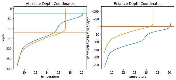
You can see the seasonal deepening/shallowing of the mixed layer in the left panel. On the right panel, the values right at the mixed-layer boundary are aligned, and the values above and below are ‘streched’. The deepening of the mixed layer is now shown with the orange line extending further into the negative numbers (meaning above the mixed layer depth).
We can now use this new coordinate to transform the whole dataset very efficiently with xgcm:
[9]:
from xgcm import Grid
import numpy as np

grid = Grid(ds, periodic=False, coords={'Z':{'center':'st_ocean'}})

# create the values to interpolate to (these are m depth relative to the mixed layer)
target_raw = np.arange(-100, 300, 20)
target = xr.DataArray(target_raw, dims=['depth_relative_to_ml'], coords={'depth_relative_to_ml':target_raw})
temp_on_z_relative = grid.transform(temp, 'Z', target , target_data=z_relative)
[10]:
temp_on_z_relative.isel(**roi, missing_dims='ignore').plot.contourf(levels=30, x='time', yincrease=False)
plt.axhline(0, color='k')
[10]:
<matplotlib.lines.Line2D at 0x7f396f7a2af0>
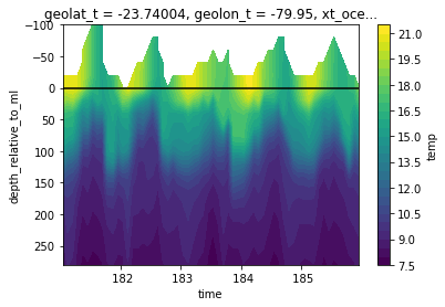
This example plot shows the time evolution of temperature relative to the mixed layer (black line). You can clearly see how the temperature values from the ‘high’ winter mixed layer are subducted into the interior while the mixed layer warms and shallows during the summer.