Antarctic bed and surface digital elevation model data

For this example we will load Bedmachine Antarctica version 1, from a google bucket and process it in the cloud https://nsidc.org/data/NSIDC-0756/versions/1

Reference:

Morlighem, M., E. Rignot, T. Binder, D. D. Blankenship, R. Drews, G. Eagles, O. Eisen, F. Ferraccioli, R. Forsberg, P. Fretwell, V. Goel, J. S. Greenbaum, H. Gudmundsson, J. Guo, V. Helm, C. Hofstede, I. Howat, A. Humbert, W. Jokat, N. B. Karlsson, W. Lee, K. Matsuoka, R. Millan, J. Mouginot, J. Paden, F. Pattyn, J. L. Roberts, S. Rosier, A. Ruppel, H. Seroussi, E. C. Smith, D. Steinhage, B. Sun, M. R. van den Broeke, T. van Ommen, M. van Wessem, and D. A. Young. 2020. Deep glacial troughs and stabilizing ridges unveiled beneath the margins of the Antarctic ice sheet, Nature Geoscience. 13. 132-137. https://doi.org/10.1038/s41561-019-0510-8

import numpy as np
import xarray as xr
import matplotlib.pyplot as plt
from intake import open_catalog

Initialize dataset

This dataset was previously (1) downloaded from the NSIDC (link above), (2) uploaded to a publicly-assessible google bucket as a zarr, (3) pointed to by an intake catalog. The latter two steps were achieved using https://github.com/ldeo-glaciology/pangeo-bedmachine/blob/master/nc_to_zarr.ipynb and https://github.com/ldeo-glaciology/pangeo-bedmachine/blob/master/intake_catalog_setup.ipynb respectively.

cat = open_catalog('https://raw.githubusercontent.com/ldeo-glaciology/pangeo-bedmachine/master/bedmachine.yaml')
ds  = cat["bedmachine"].to_dask()
ds

<xarray.Dataset>
Dimensions:    (x: 13333, y: 13333)
Coordinates:
  * x          (x) int32 -3333000 -3332500 -3332000 ... 3332000 3332500 3333000
  * y          (y) int32 3333000 3332500 3332000 ... -3332000 -3332500 -3333000
Data variables:
    bed        (y, x) float32 dask.array<chunksize=(3000, 3000), meta=np.ndarray>
    errbed     (y, x) float32 dask.array<chunksize=(3000, 3000), meta=np.ndarray>
    firn       (y, x) float32 dask.array<chunksize=(3000, 3000), meta=np.ndarray>
    geoid      (y, x) int16 dask.array<chunksize=(3000, 3000), meta=np.ndarray>
    mask       (y, x) int8 dask.array<chunksize=(3000, 3000), meta=np.ndarray>
    source     (y, x) int8 dask.array<chunksize=(3000, 3000), meta=np.ndarray>
    surface    (y, x) float32 dask.array<chunksize=(3000, 3000), meta=np.ndarray>
    thickness  (y, x) float32 dask.array<chunksize=(3000, 3000), meta=np.ndarray>
Attributes:
    Author:                                 Mathieu Morlighem
    Conventions:                            CF-1.7
    Data_citation:                          Morlighem M. et al., (2019), Deep...
    Notes:                                  Data processed at the Department ...
    Projection:                             Polar Stereographic South (71S,0E)
    Title:                                  BedMachine Antarctica
    false_easting:                          [0.0]
    false_northing:                         [0.0]
    grid_mapping_name:                      polar_stereographic
    ice_density (kg m-3):                   [917.0]
    inverse_flattening:                     [298.2794050428205]
    latitude_of_projection_origin:          [-90.0]
    license:                                No restrictions on access or use
    no_data:                                [-9999.0]
    nx:                                     [13333.0]
    ny:                                     [13333.0]
    proj4:                                  +init=epsg:3031
    sea_water_density (kg m-3):             [1027.0]
    semi_major_axis:                        [6378273.0]
    spacing:                                [500]
    standard_parallel:                      [-71.0]
    straight_vertical_longitude_from_pole:  [0.0]
    version:                                05-Nov-2019 (v1.38)
    xmin:                                   [-3333000]
    ymax:                                   [3333000]

check how big the dataset is

(its not very large - only 4.2 GB - but still slower to download and process in a conventional way that in pangeo)

ds.nbytes/1e9

4.26656

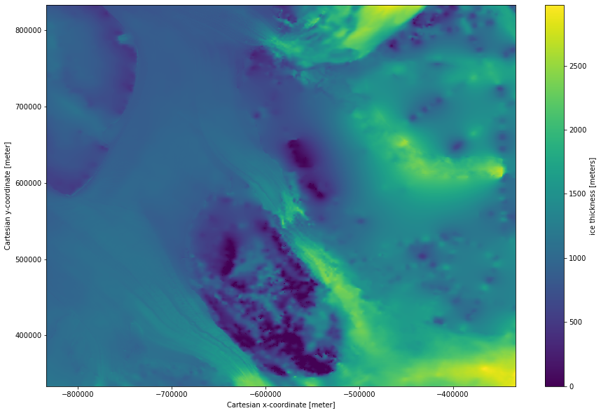
plot some of the data to take a look at one of the fields

Subset and plot the ice thickness

ds.thickness.isel(x=slice(5000,6000), y = slice(5000,6000)).plot(size = 10);

<matplotlib.collections.QuadMesh at 0x7fe72ea968e0>

start a cluster to do some fast processing of this relatively small dataset

from dask.distributed import Client
import dask_gateway

gateway = dask_gateway.Gateway()
cluster = gateway.new_cluster()

cluster.scale(4)
client = Client(cluster)
cluster

To view the dask scheduler dashboard either click the link above, or copy the link in to the serach bar in the dask tab on the right, prefixing it with https://us-central1-b.gcp.pangeo.io/ - then you get access to all the tool and they can be docked in this window.

do a simple calculation that requires three of the dataarrays in their entirety

compute the mean thickness from the difference between surface and bed heights and compare that to the mean of the thickness datarray

diff = ds.surface - ds.bed   # take the difference between the surface and the bed
ice_surf_bed_diff = diff.where(ds.mask!=0)   # only consider places where there is ice (i.e. where mask is not equal to zero)
mean_surf_bed_diff = ice_surf_bed_diff.mean()  # compute the mean

this hasnt done any computation, it has just prepared the computation.

surf_bed_diff is just a place holder for a 13333x13333 array

mean_surf_bed_diff

<xarray.DataArray ()>
dask.array<mean_agg-aggregate, shape=(), dtype=float32, chunksize=(), chunktype=numpy.ndarray>

and mt1 is just a place holder for a sinlge value (the mean of hte difference)

mean_surf_bed_diff

<xarray.DataArray ()>
dask.array<mean_agg-aggregate, shape=(), dtype=float32, chunksize=(), chunktype=numpy.ndarray>

execute the computation

.load() is one of several dask commands that causes the computation to be executed.

%%time
mean_surf_bed_diff.load()

CPU times: user 155 ms, sys: 39.3 ms, total: 195 ms
Wall time: 2min 59s

<xarray.DataArray ()>
array(1944.0841, dtype=float32)

note that if you call mt1.load() again it generally will not waste time computing the result again as it has it stored in the cluster memory (unless something has cleared in the meantime since the block above was called, e.g., del mean_surf_bed_diff). It just returns the result again.

%%time
mean_surf_bed_diff.load()

CPU times: user 105 µs, sys: 24 µs, total: 129 µs
Wall time: 138 µs

<xarray.DataArray ()>
array(1944.0841, dtype=float32)

now compare this to the mean of the thickness field

%%time
mt2 = ds.thickness.where(ds.mask!=0).mean().load()
mt2

CPU times: user 17.6 ms, sys: 3.13 ms, total: 20.7 ms
Wall time: 1.7 s

<xarray.DataArray 'thickness' ()>
array(1916.2861, dtype=float32)

its close but not exactly the same, which is to be expected.

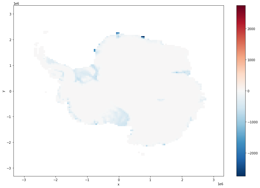
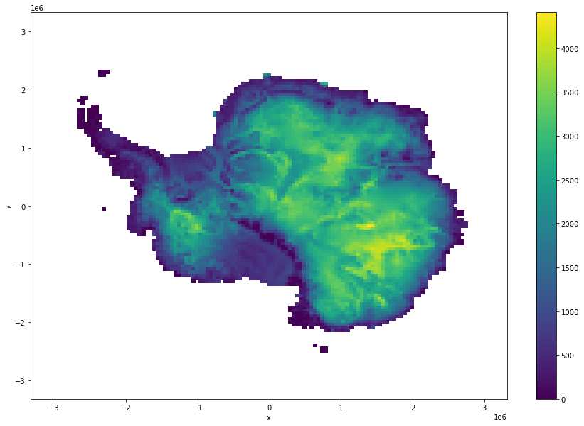
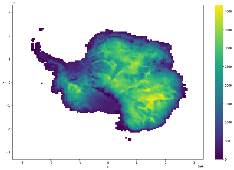
Make some plots, making use of coarsen.

Plot the two thickness field and the differnece between them, making use of course, so that we dont need to download the whole dataset just for these plots.

ice_surf_bed_diff.coarsen(x=100,y=100,boundary="trim").mean().plot(size = 10)

<matplotlib.collections.QuadMesh at 0x7fe72e9f68e0>

ds.thickness.where(ds.mask!=0).coarsen(x=100,y=100,boundary="trim").mean().plot(size = 10)

<matplotlib.collections.QuadMesh at 0x7fe705c10c40>

mismatch = ds.thickness - ice_surf_bed_diff
mismatch.where(ds.mask!=0).coarsen(x=100,y=100,boundary="trim").mean().plot(size = 10)

<matplotlib.collections.QuadMesh at 0x7fe705b56820>