
Ice sheet model output
This notebook demonstrates how to load, process and plot output from an ensemble of simulations of the Antarctic Ice Sheet from the last interglacial to present.
2020 by Torsten Albrecht (torsten.albrecht@pik-potsdam.de) | Potsdam Institute for Climate Impact Research (PIK)
data: Albrecht, Torsten (2019): PISM parameter ensemble analysis of Antarctic Ice Sheet glacial cycle simulations. PANGAEA, https://doi.pangaea.de/10.1594/PANGAEA.909728
More details on the ensemble can be found here.
[1]:
# load a package called intake, which is used to load the data.
import intake
1. Lazily load the model data
Selected outputs from the model ensemble are stored in two zarr directories in the google cloud. The data are cataloged in intake catalogs to simplify loading.
The zarr directory ‘present’ contains fields that describe the state of each ensemble member at the end of the simulation, i.e. the simulated ‘present-day’ state.
The zarr directory ‘mask_score_time_series’ contains time series of an integer mask (indicating ice-free/grounded/floating/ocean) for each ensemble member.
The cell below first loads the intake catalog from a github repo, then loads data from these two zarr directories in turn. However, it loads the data ‘lazily’, meaning that the data does not enter into memory untill we need them to, and ‘present’ and ‘mask_score_time_series’ are really just pointers to where the data are held, so that when we want to do a computation the machine will know where to look.
[2]:
# load the intake catalog
cat = intake.open_catalog('https://raw.githubusercontent.com/ldeo-glaciology/pangeo-pismpaleo/main/paleopism.yaml')

# load each of the zarr diretories contained in the intake catalog
present  = cat["present"].to_dask()
mask_score_time_series  = cat["mask_score_time_series"].to_dask()
2. Let’s take a look at the resulting xarrays
present
dimensions
present is a 7-dimensional xarray:
It has dimensions corresponding to each of the four ensemble parameters: par_esia, par_ppq, par_prec and par_visc
It has one time dimension, but this is only one element long so it can be mostly ignored.
It has two spatial dimensions, x and y.
Each dimensionn has a corresponding coordinate, which provides the values for the dimensions (i.e. the parameter values, the UPS X and Y). There is also an addition pair of coordinates called lat and lon, which provide the geographic positions of the grid cells.
variables
It contains variables corresponding to ice thickness (thk), ice surface elevation (usurf), ice speed (velsurf_mag), an integer mask (mask; indicating ice-free/grounded/floating/ocean), and bedrock uplift rate (dbdt).
It also contains a variable called ‘score’, which quantifies how well that ensemble member matched observationally constrain ice-sheet extent.
the xarray can be viewed by simply typing it name and executing the cell:
[3]:
present
[3]:
<xarray.Dataset>
Dimensions:      (par_esia: 4, par_ppq: 4, par_prec: 4, par_visc: 4, time: 1, x: 381, y: 381)
Coordinates:
    lat          (y, x) float64 dask.array<chunksize=(191, 191), meta=np.ndarray>
    lon          (y, x) float64 dask.array<chunksize=(191, 191), meta=np.ndarray>
  * par_esia     (par_esia) float64 1.0 2.0 4.0 7.0
  * par_ppq      (par_ppq) float64 0.25 0.5 0.75 1.0
  * par_prec     (par_prec) float64 0.02 0.05 0.07 0.1
  * par_visc     (par_visc) float64 1e+20 5e+20 2.5e+21 1e+22
  * time         (time) float64 50.0
  * x            (x) float64 -3.04e+06 -3.024e+06 ... 3.024e+06 3.04e+06
  * y            (y) float64 -3.04e+06 -3.024e+06 ... 3.024e+06 3.04e+06
Data variables:
    dbdt         (time, y, x, par_esia, par_ppq, par_prec, par_visc) float64 dask.array<chunksize=(1, 381, 381, 1, 4, 4, 4), meta=np.ndarray>
    index        (par_esia, par_ppq, par_prec, par_visc) int64 dask.array<chunksize=(4, 4, 4, 4), meta=np.ndarray>
    mask         (time, y, x, par_esia, par_ppq, par_prec, par_visc) int8 dask.array<chunksize=(1, 381, 381, 1, 4, 4, 4), meta=np.ndarray>
    score        (par_esia, par_ppq, par_prec, par_visc) float64 dask.array<chunksize=(4, 4, 4, 4), meta=np.ndarray>
    thk          (time, y, x, par_esia, par_ppq, par_prec, par_visc) float64 dask.array<chunksize=(1, 381, 381, 1, 4, 4, 4), meta=np.ndarray>
    topg         (time, y, x, par_esia, par_ppq, par_prec, par_visc) float64 dask.array<chunksize=(1, 381, 381, 1, 4, 4, 4), meta=np.ndarray>
    usurf        (time, y, x, par_esia, par_ppq, par_prec, par_visc) float32 dask.array<chunksize=(1, 381, 381, 1, 4, 4, 4), meta=np.ndarray>
    velsurf_mag  (time, y, x, par_esia, par_ppq, par_prec, par_visc) float32 dask.array<chunksize=(1, 381, 381, 1, 4, 4, 4), meta=np.ndarray>
Attributes:
    NCO:              4.6.8
    command:           /p/tmp/albrecht/pism18/pismOut/pism_paleo/pism1.0_pale...
    history:          Thu Dec  5 15:34:39 2019: ncatted -O -a history,global,...
parameter_space: {'visc': [1e+20, 5e+20, 2.5e+21, 1e+22], 'sia_e': [1.0,...- par_esia: 4
- par_ppq: 4
- par_prec: 4
- par_visc: 4
- time: 1
- x: 381
- y: 381
- lat(y, x)float64dask.array<chunksize=(191, 191), meta=np.ndarray>
- bounds :
- lat_bnds
- long_name :
- latitude
- pism_intent :
- mapping
- standard_name :
- latitude
- units :
- degree_north
- valid_range :
- [-90.0, 90.0]
Array Chunk Bytes 1.16 MB 291.85 kB Shape (381, 381) (191, 191) Count 5 Tasks 4 Chunks Type float64 numpy.ndarray - lon(y, x)float64dask.array<chunksize=(191, 191), meta=np.ndarray>
- bounds :
- lon_bnds
- long_name :
- longitude
- pism_intent :
- mapping
- standard_name :
- longitude
- units :
- degree_east
- valid_range :
- [-180.0, 180.0]
Array Chunk Bytes 1.16 MB 291.85 kB Shape (381, 381) (191, 191) Count 5 Tasks 4 Chunks Type float64 numpy.ndarray - par_esia(par_esia)float641.0 2.0 4.0 7.0
array([1., 2., 4., 7.])
- par_ppq(par_ppq)float640.25 0.5 0.75 1.0
array([0.25, 0.5 , 0.75, 1. ])
- par_prec(par_prec)float640.02 0.05 0.07 0.1
array([0.02, 0.05, 0.07, 0.1 ])
- par_visc(par_visc)float641e+20 5e+20 2.5e+21 1e+22
array([1.0e+20, 5.0e+20, 2.5e+21, 1.0e+22])
- time(time)float6450.0
array([50.])
- x(x)float64-3.04e+06 -3.024e+06 ... 3.04e+06
- axis :
- X
- long_name :
- X-coordinate in Cartesian system
- spacing_meters :
- 16000.0
- standard_name :
- projection_x_coordinate
- units :
- m
array([-3040000., -3024000., -3008000., ..., 3008000., 3024000., 3040000.])
- y(y)float64-3.04e+06 -3.024e+06 ... 3.04e+06
- axis :
- Y
- long_name :
- Y-coordinate in Cartesian system
- spacing_meters :
- 16000.0
- standard_name :
- projection_y_coordinate
- units :
- m
array([-3040000., -3024000., -3008000., ..., 3008000., 3024000., 3040000.])
- dbdt(time, y, x, par_esia, par_ppq, par_prec, par_visc)float64dask.array<chunksize=(1, 381, 381, 1, 4, 4, 4), meta=np.ndarray>
- long_name :
- bedrock uplift rate
- pism_intent :
- model_state
- standard_name :
- tendency_of_bedrock_altitude
- units :
- mm year-1
Array Chunk Bytes 297.29 MB 74.32 MB Shape (1, 381, 381, 4, 4, 4, 4) (1, 381, 381, 1, 4, 4, 4) Count 5 Tasks 4 Chunks Type float64 numpy.ndarray - index(par_esia, par_ppq, par_prec, par_visc)int64dask.array<chunksize=(4, 4, 4, 4), meta=np.ndarray>
Array Chunk Bytes 2.05 kB 2.05 kB Shape (4, 4, 4, 4) (4, 4, 4, 4) Count 2 Tasks 1 Chunks Type int64 numpy.ndarray - mask(time, y, x, par_esia, par_ppq, par_prec, par_visc)int8dask.array<chunksize=(1, 381, 381, 1, 4, 4, 4), meta=np.ndarray>
- flag_meanings :
- ice_free_bedrock grounded_ice floating_ice ice_free_ocean
- flag_values :
- [0, 2, 3, 4]
- long_name :
- ice-type (ice-free/grounded/floating/ocean) integer mask
- pism_intent :
- diagnostic
- units :
Array Chunk Bytes 37.16 MB 9.29 MB Shape (1, 381, 381, 4, 4, 4, 4) (1, 381, 381, 1, 4, 4, 4) Count 5 Tasks 4 Chunks Type int8 numpy.ndarray - score(par_esia, par_ppq, par_prec, par_visc)float64dask.array<chunksize=(4, 4, 4, 4), meta=np.ndarray>
Array Chunk Bytes 2.05 kB 2.05 kB Shape (4, 4, 4, 4) (4, 4, 4, 4) Count 2 Tasks 1 Chunks Type float64 numpy.ndarray - thk(time, y, x, par_esia, par_ppq, par_prec, par_visc)float64dask.array<chunksize=(1, 381, 381, 1, 4, 4, 4), meta=np.ndarray>
- long_name :
- land ice thickness
- pism_intent :
- model_state
- standard_name :
- land_ice_thickness
- units :
- m
- valid_min :
- 0.0
Array Chunk Bytes 297.29 MB 74.32 MB Shape (1, 381, 381, 4, 4, 4, 4) (1, 381, 381, 1, 4, 4, 4) Count 5 Tasks 4 Chunks Type float64 numpy.ndarray - topg(time, y, x, par_esia, par_ppq, par_prec, par_visc)float64dask.array<chunksize=(1, 381, 381, 1, 4, 4, 4), meta=np.ndarray>
- long_name :
- bedrock surface elevation
- pism_intent :
- model_state
- standard_name :
- bedrock_altitude
- units :
- m
Array Chunk Bytes 297.29 MB 74.32 MB Shape (1, 381, 381, 4, 4, 4, 4) (1, 381, 381, 1, 4, 4, 4) Count 5 Tasks 4 Chunks Type float64 numpy.ndarray - usurf(time, y, x, par_esia, par_ppq, par_prec, par_visc)float32dask.array<chunksize=(1, 381, 381, 1, 4, 4, 4), meta=np.ndarray>
- long_name :
- ice upper surface elevation
- pism_intent :
- diagnostic
- standard_name :
- surface_altitude
- units :
- m
Array Chunk Bytes 148.64 MB 37.16 MB Shape (1, 381, 381, 4, 4, 4, 4) (1, 381, 381, 1, 4, 4, 4) Count 5 Tasks 4 Chunks Type float32 numpy.ndarray - velsurf_mag(time, y, x, par_esia, par_ppq, par_prec, par_visc)float32dask.array<chunksize=(1, 381, 381, 1, 4, 4, 4), meta=np.ndarray>
- long_name :
- magnitude of horizontal velocity of ice at ice surface
- pism_intent :
- diagnostic
- units :
- m year-1
- valid_min :
- 0.0
Array Chunk Bytes 148.64 MB 37.16 MB Shape (1, 381, 381, 4, 4, 4, 4) (1, 381, 381, 1, 4, 4, 4) Count 5 Tasks 4 Chunks Type float32 numpy.ndarray
- NCO :
- 4.6.8
- command :
- /p/tmp/albrecht/pism18/pismOut/pism_paleo/pism1.0_paleo06_6000/./bin/pismr -i /p/tmp/albrecht/pism18/pismOut/forcing/forcing2533_TPSO/results/snap_forcing_16km_210000yrs.nc_-125000.000.nc -config /p/tmp/albrecht/pism18/pismOut/pism_paleo/pism1.0_paleo06_6000/pism_config_default.nc -config_override /p/tmp/albrecht/pism18/pismOut/pism_paleo/pism1.0_paleo06_6000/pism_config_override.nc -ys -125000 -ye 50 -o paleo.nc -o_size big -o_order zyx -backup_interval 3.0 -verbose 2 -options_left -atmosphere pik_temp,delta_T,paleo_precip,lapse_rate -temp_era_interim_lon -atmosphere_pik_temp_file /p/tmp/albrecht/pism18/pismOut/forcing/forcing2533_TPSO/results/snap_forcing_16km_210000yrs.nc_-125000.000.nc -atmosphere_delta_T_file /p/tmp/albrecht/pism18/pismInput/timeseries_edc-wdc_temp.nc -atmosphere_paleo_precip_file /p/tmp/albrecht/pism18/pismInput/timeseries_edc-wdc_temp.nc -atmosphere_lapse_rate_file /p/tmp/albrecht/pism18/pismInput/bedmap2_albmap_racmo_wessem_schmidtko_11+12_uplift_velrignot_bheatflx_lgmokill_fttmask_16km.nc -temp_lapse_rate 0.0 -precip_lapse_scaling -precip_scale_factor 0.554 -surface pdd -ocean cavity,delta_SL -ocean_cavity_file /p/tmp/albrecht/pism18/pismInput/schmidtko14_edc-wdc_oceantemp_basins_response_fit_16km.nc -ocean_delta_SL_file /p/tmp/albrecht/pism18/pismInput/imbrie06peltier15_sl_ramp205ka.nc -exclude_icerises -number_of_basins 20 -continental_shelf_depth -2500 -gamma_T 1.0e-5 -overturning_coeff 0.8e6 -calving eigen_calving,thickness_calving,ocean_kill -ocean_kill_file /p/tmp/albrecht/pism18/pismInput/bedmap2_albmap_racmo_wessem_schmidtko_11+12_uplift_velrignot_bheatflx_lgmokill_fttmask_16km.nc -ocean_kill_mask -bed_def lc -hydrology null -include_ocean_load -subgl -yield_stress mohr_coulomb -pseudo_plastic -pik -stress_balance ssa+sia -ssa_method fd -sia_flow_law gpbld -ssa_flow_law gpbld -extra_file extra_paleo.nc -extra_times -125000:1000:0 -extra_vars velbar_mag,cell_area,mask,dbdt,topg,thk,usurf,tauc,ice_surface_temp,climatic_mass_balance,bmelt -save_file snapshots -save_times -125000:5000:0 -save_split -save_size medium -ts_times -125000:1:50 -ts_file timeseries.nc /p/tmp/albrecht/pism18/pismOut/pism_paleo/pism1.0_paleo06_6000/./bin/pismr -i /p/tmp/albrecht/pism18/pismOut/forcing/forcing2533_TPSO/results/snap_forcing_16km_210000yrs.nc_-125000.000.nc -config /p/tmp/albrecht/pism18/pismOut/pism_paleo/pism1.0_paleo06_6000/pism_config_default.nc -config_override /p/tmp/albrecht/pism18/pismOut/pism_paleo/pism1.0_paleo06_6000/pism_config_override.nc -ys -125000 -ye 50 -o paleo.nc -o_size big -o_order zyx -backup_interval 3.0 -verbose 2 -options_left -atmosphere pik_temp,delta_T,paleo_precip,lapse_rate -temp_era_interim_lon -atmosphere_pik_temp_file /p/tmp/albrecht/pism18/pismOut/forcing/forcing2533_TPSO/results/snap_forcing_16km_210000yrs.nc_-125000.000.nc -atmosphere_delta_T_file /p/tmp/albrecht/pism18/pismInput/timeseries_edc-wdc_temp.nc -atmosphere_paleo_precip_file /p/tmp/albrecht/pism18/pismInput/timeseries_edc-wdc_temp.nc -atmosphere_lapse_rate_file /p/tmp/albrecht/pism18/pismInput/bedmap2_albmap_racmo_wessem_schmidtko_11+12_uplift_velrignot_bheatflx_lgmokill_fttmask_16km.nc -temp_lapse_rate 0.0 -precip_lapse_scaling -precip_scale_factor 0.554 -surface pdd -ocean cavity,delta_SL -ocean_cavity_file /p/tmp/albrecht/pism18/pismInput/schmidtko14_edc-wdc_oceantemp_basins_response_fit_16km.nc -ocean_delta_SL_file /p/tmp/albrecht/pism18/pismInput/imbrie06peltier15_sl_ramp205ka.nc -exclude_icerises -number_of_basins 20 -continental_shelf_depth -2500 -gamma_T 1.0e-5 -overturning_coeff 0.8e6 -calving eigen_calving,thickness_calving,ocean_kill -ocean_kill_file /p/tmp/albrecht/pism18/pismInput/bedmap2_albmap_racmo_wessem_schmidtko_11+12_uplift_velrignot_bheatflx_lgmokill_fttmask_16km.nc -ocean_kill_mask -bed_def lc -hydrology null -include_ocean_load -subgl -yield_stress mohr_coulomb -pseudo_plastic -pik -stress_balance ssa+sia -ssa_method fd -sia_flow_law gpbld -ssa_flow_law gpbld -extra_file extra_paleo.nc -extra_times -125000:1000:0 -extra_vars velbar_mag,cell_area,mask,dbdt,topg,thk,usurf,tauc,ice_surface_temp,climatic_mass_balance,bmelt -save_file snapshots -save_times -125000:5000:0 -save_split -save_size medium -ts_times -125000:1:50 -ts_file timeseries.nc
- history :
- Thu Dec 5 15:34:39 2019: ncatted -O -a history,global,d,, /p/tmp/albrecht/paleo_ensemble/datapub/model_data/pism1.0_paleo06_6000/paleo.nc
- parameter_space :
- {'visc': [1e+20, 5e+20, 2.5e+21, 1e+22], 'sia_e': [1.0, 2.0, 4.0, 7.0], 'prec': [0.02, 0.05, 0.07, 0.1], 'ppq': [0.25, 0.5, 0.75, 1.0]}
mask_score_time_series is also 7-dimensional xarray:
It has the same dimensions as present (above), but in len(mask_score_time_series.time) returns 125, indicating that this dataset has multiple time slices.
[4]:
mask_score_time_series
[4]:
<xarray.Dataset>
Dimensions:   (par_esia: 4, par_ppq: 4, par_prec: 4, par_visc: 4, time: 125, x: 381, y: 381)
Coordinates:
  * par_esia  (par_esia) float64 1.0 2.0 4.0 7.0
  * par_ppq   (par_ppq) float64 0.25 0.5 0.75 1.0
  * par_prec  (par_prec) float64 0.02 0.05 0.07 0.1
  * par_visc  (par_visc) float64 1e+20 5e+20 2.5e+21 1e+22
  * time      (time) float64 -1.24e+05 -1.23e+05 -1.22e+05 ... -2e+03 -1e+03 0.0
  * x         (x) float64 -3.04e+06 -3.024e+06 -3.008e+06 ... 3.024e+06 3.04e+06
  * y         (y) float64 -3.04e+06 -3.024e+06 -3.008e+06 ... 3.024e+06 3.04e+06
Data variables:
    index     (par_esia, par_ppq, par_prec, par_visc) int64 dask.array<chunksize=(4, 4, 4, 4), meta=np.ndarray>
    mask      (time, y, x, par_esia, par_ppq, par_prec, par_visc) int8 dask.array<chunksize=(125, 381, 381, 1, 4, 4, 4), meta=np.ndarray>
    score     (time, par_esia, par_ppq, par_prec, par_visc) float64 dask.array<chunksize=(125, 4, 4, 4, 4), meta=np.ndarray>
Attributes:
    NCO:              4.6.8
    command:           /p/tmp/albrecht/pism18/pismOut/pism_paleo/pism1.0_pale...
    history:          Thu Dec  5 16:44:54 2019: ncatted -O -a history,global,...
parameter_space: {'visc': [1e+20, 5e+20, 2.5e+21, 1e+22], 'sia_e': [1.0,...- par_esia: 4
- par_ppq: 4
- par_prec: 4
- par_visc: 4
- time: 125
- x: 381
- y: 381
- par_esia(par_esia)float641.0 2.0 4.0 7.0
array([1., 2., 4., 7.])
- par_ppq(par_ppq)float640.25 0.5 0.75 1.0
array([0.25, 0.5 , 0.75, 1. ])
- par_prec(par_prec)float640.02 0.05 0.07 0.1
array([0.02, 0.05, 0.07, 0.1 ])
- par_visc(par_visc)float641e+20 5e+20 2.5e+21 1e+22
array([1.0e+20, 5.0e+20, 2.5e+21, 1.0e+22])
- time(time)float64-1.24e+05 -1.23e+05 ... -1e+03 0.0
array([-124000., -123000., -122000., -121000., -120000., -119000., -118000., -117000., -116000., -115000., -114000., -113000., -112000., -111000., -110000., -109000., -108000., -107000., -106000., -105000., -104000., -103000., -102000., -101000., -100000., -99000., -98000., -97000., -96000., -95000., -94000., -93000., -92000., -91000., -90000., -89000., -88000., -87000., -86000., -85000., -84000., -83000., -82000., -81000., -80000., -79000., -78000., -77000., -76000., -75000., -74000., -73000., -72000., -71000., -70000., -69000., -68000., -67000., -66000., -65000., -64000., -63000., -62000., -61000., -60000., -59000., -58000., -57000., -56000., -55000., -54000., -53000., -52000., -51000., -50000., -49000., -48000., -47000., -46000., -45000., -44000., -43000., -42000., -41000., -40000., -39000., -38000., -37000., -36000., -35000., -34000., -33000., -32000., -31000., -30000., -29000., -28000., -27000., -26000., -25000., -24000., -23000., -22000., -21000., -20000., -19000., -18000., -17000., -16000., -15000., -14000., -13000., -12000., -11000., -10000., -9000., -8000., -7000., -6000., -5000., -4000., -3000., -2000., -1000., 0.]) - x(x)float64-3.04e+06 -3.024e+06 ... 3.04e+06
- axis :
- X
- long_name :
- X-coordinate in Cartesian system
- spacing_meters :
- 16000.0
- standard_name :
- projection_x_coordinate
- units :
- m
array([-3040000., -3024000., -3008000., ..., 3008000., 3024000., 3040000.])
- y(y)float64-3.04e+06 -3.024e+06 ... 3.04e+06
- axis :
- Y
- long_name :
- Y-coordinate in Cartesian system
- spacing_meters :
- 16000.0
- standard_name :
- projection_y_coordinate
- units :
- m
array([-3040000., -3024000., -3008000., ..., 3008000., 3024000., 3040000.])
- index(par_esia, par_ppq, par_prec, par_visc)int64dask.array<chunksize=(4, 4, 4, 4), meta=np.ndarray>
Array Chunk Bytes 2.05 kB 2.05 kB Shape (4, 4, 4, 4) (4, 4, 4, 4) Count 2 Tasks 1 Chunks Type int64 numpy.ndarray - mask(time, y, x, par_esia, par_ppq, par_prec, par_visc)int8dask.array<chunksize=(125, 381, 381, 1, 4, 4, 4), meta=np.ndarray>
- coordinates :
- lat lon
- flag_meanings :
- ice_free_bedrock grounded_ice floating_ice ice_free_ocean
- flag_values :
- [0, 2, 3, 4]
- long_name :
- ice-type (ice-free/grounded/floating/ocean) integer mask
- pism_intent :
- diagnostic
- units :
Array Chunk Bytes 4.65 GB 1.16 GB Shape (125, 381, 381, 4, 4, 4, 4) (125, 381, 381, 1, 4, 4, 4) Count 5 Tasks 4 Chunks Type int8 numpy.ndarray - score(time, par_esia, par_ppq, par_prec, par_visc)float64dask.array<chunksize=(125, 4, 4, 4, 4), meta=np.ndarray>
Array Chunk Bytes 256.00 kB 256.00 kB Shape (125, 4, 4, 4, 4) (125, 4, 4, 4, 4) Count 2 Tasks 1 Chunks Type float64 numpy.ndarray
- NCO :
- 4.6.8
- command :
- /p/tmp/albrecht/pism18/pismOut/pism_paleo/pism1.0_paleo06_6000/./bin/pismr -i /p/tmp/albrecht/pism18/pismOut/forcing/forcing2533_TPSO/results/snap_forcing_16km_210000yrs.nc_-125000.000.nc -config /p/tmp/albrecht/pism18/pismOut/pism_paleo/pism1.0_paleo06_6000/pism_config_default.nc -config_override /p/tmp/albrecht/pism18/pismOut/pism_paleo/pism1.0_paleo06_6000/pism_config_override.nc -ys -125000 -ye 50 -o paleo.nc -o_size big -o_order zyx -backup_interval 3.0 -verbose 2 -options_left -atmosphere pik_temp,delta_T,paleo_precip,lapse_rate -temp_era_interim_lon -atmosphere_pik_temp_file /p/tmp/albrecht/pism18/pismOut/forcing/forcing2533_TPSO/results/snap_forcing_16km_210000yrs.nc_-125000.000.nc -atmosphere_delta_T_file /p/tmp/albrecht/pism18/pismInput/timeseries_edc-wdc_temp.nc -atmosphere_paleo_precip_file /p/tmp/albrecht/pism18/pismInput/timeseries_edc-wdc_temp.nc -atmosphere_lapse_rate_file /p/tmp/albrecht/pism18/pismInput/bedmap2_albmap_racmo_wessem_schmidtko_11+12_uplift_velrignot_bheatflx_lgmokill_fttmask_16km.nc -temp_lapse_rate 0.0 -precip_lapse_scaling -precip_scale_factor 0.554 -surface pdd -ocean cavity,delta_SL -ocean_cavity_file /p/tmp/albrecht/pism18/pismInput/schmidtko14_edc-wdc_oceantemp_basins_response_fit_16km.nc -ocean_delta_SL_file /p/tmp/albrecht/pism18/pismInput/imbrie06peltier15_sl_ramp205ka.nc -exclude_icerises -number_of_basins 20 -continental_shelf_depth -2500 -gamma_T 1.0e-5 -overturning_coeff 0.8e6 -calving eigen_calving,thickness_calving,ocean_kill -ocean_kill_file /p/tmp/albrecht/pism18/pismInput/bedmap2_albmap_racmo_wessem_schmidtko_11+12_uplift_velrignot_bheatflx_lgmokill_fttmask_16km.nc -ocean_kill_mask -bed_def lc -hydrology null -include_ocean_load -subgl -yield_stress mohr_coulomb -pseudo_plastic -pik -stress_balance ssa+sia -ssa_method fd -sia_flow_law gpbld -ssa_flow_law gpbld -extra_file extra_paleo.nc -extra_times -125000:1000:0 -extra_vars velbar_mag,cell_area,mask,dbdt,topg,thk,usurf,tauc,ice_surface_temp,climatic_mass_balance,bmelt -save_file snapshots -save_times -125000:5000:0 -save_split -save_size medium -ts_times -125000:1:50 -ts_file timeseries.nc
- history :
- Thu Dec 5 16:44:54 2019: ncatted -O -a history,global,d,, /p/tmp/albrecht/paleo_ensemble/datapub/model_data/pism1.0_paleo06_6000/extra_paleo_mask.nc
- parameter_space :
- {'visc': [1e+20, 5e+20, 2.5e+21, 1e+22], 'sia_e': [1.0, 2.0, 4.0, 7.0], 'prec': [0.02, 0.05, 0.07, 0.1], 'ppq': [0.25, 0.5, 0.75, 1.0]}
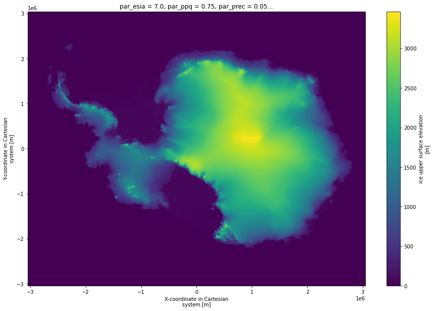
3. Let’s plot the ice velocity field of one ensemble members
To select one of the ensemble members you need to choose which of the different choices for each paramater you want to plot. This example picks this randomly.
[5]:
present.usurf.isel(par_esia=3,par_ppq = 2, par_prec= 1,par_visc = 2).plot(size = 10)
[5]:
<matplotlib.collections.QuadMesh at 0x7f5964493520>
4. Do some calculations using all ensemble members
xarrays are great for dealing with high-dimensional data like this ensemble.
4a. calculate the standard deviation of thickness across the ensemble for each location
[6]:
mean_std = present.thk.std({'par_esia','par_visc','par_ppq','par_prec'},keep_attrs=True)
mean_std.plot(size = 10)
[6]:
<matplotlib.collections.QuadMesh at 0x7f59643717f0>
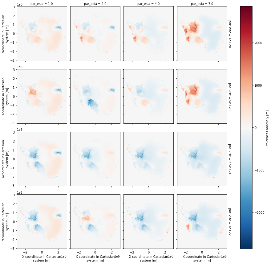
4b. Compute anomalies
Compute the difference between several ensemble members and the ensemble-wide mean computed above, then plot the results as an array of plots.
[7]:
mean_thk = present.thk.mean({'par_esia','par_visc','par_ppq','par_prec'},keep_attrs=True)
thickness_anomaly = (present.thk.isel(par_ppq=3,par_prec=2)-mean_thk)
thickness_anomaly.attrs['long_name'] = 'thickness anomaly'
thickness_anomaly.attrs['units'] = 'm'
thickness_anomaly.plot(x='x',y='y',col='par_esia',row='par_visc');
[7]:
<xarray.plot.facetgrid.FacetGrid at 0x7f59645f4700>
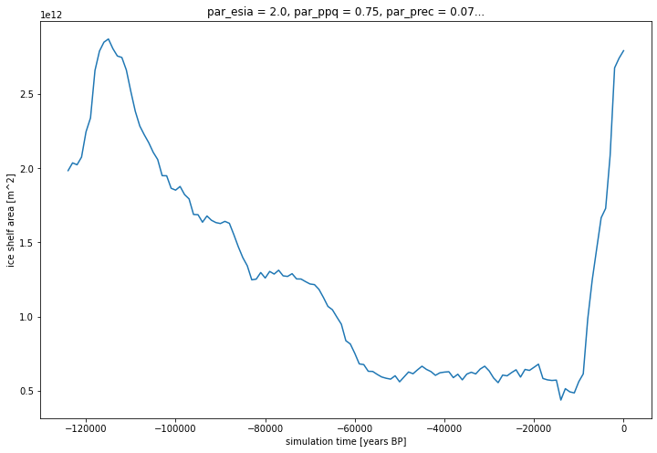
5. Plot the time slice data.
5a. plot a time series of ice shelf area
[8]:
cellArea = mask_score_time_series.x.attrs['spacing_meters'] * mask_score_time_series.y.attrs['spacing_meters']
[9]:
import xarray as xr
ice_shelf_area = (xr.where(mask_score_time_series.mask.isel(par_esia=1, par_ppq=2, par_prec=2, par_visc=3) == 3 ,1 ,0 ).sum(['x','y'])*cellArea)
ice_shelf_area.attrs['units'] = 'm^2'
ice_shelf_area.attrs['long_name'] = 'ice shelf area'
ice_shelf_area.time.attrs['long_name'] = 'simulation time'
ice_shelf_area.time.attrs['units'] = 'years BP'
p = ice_shelf_area.plot(size=8)
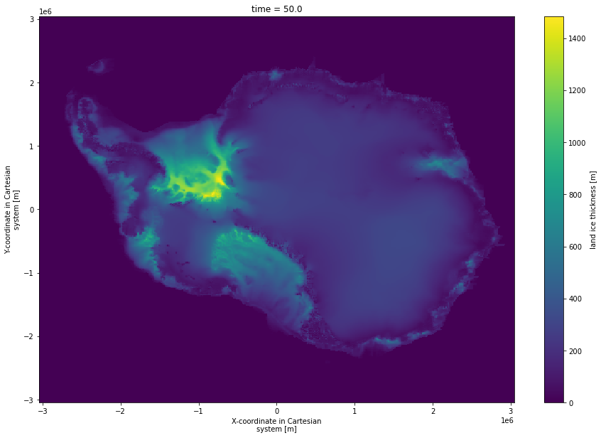
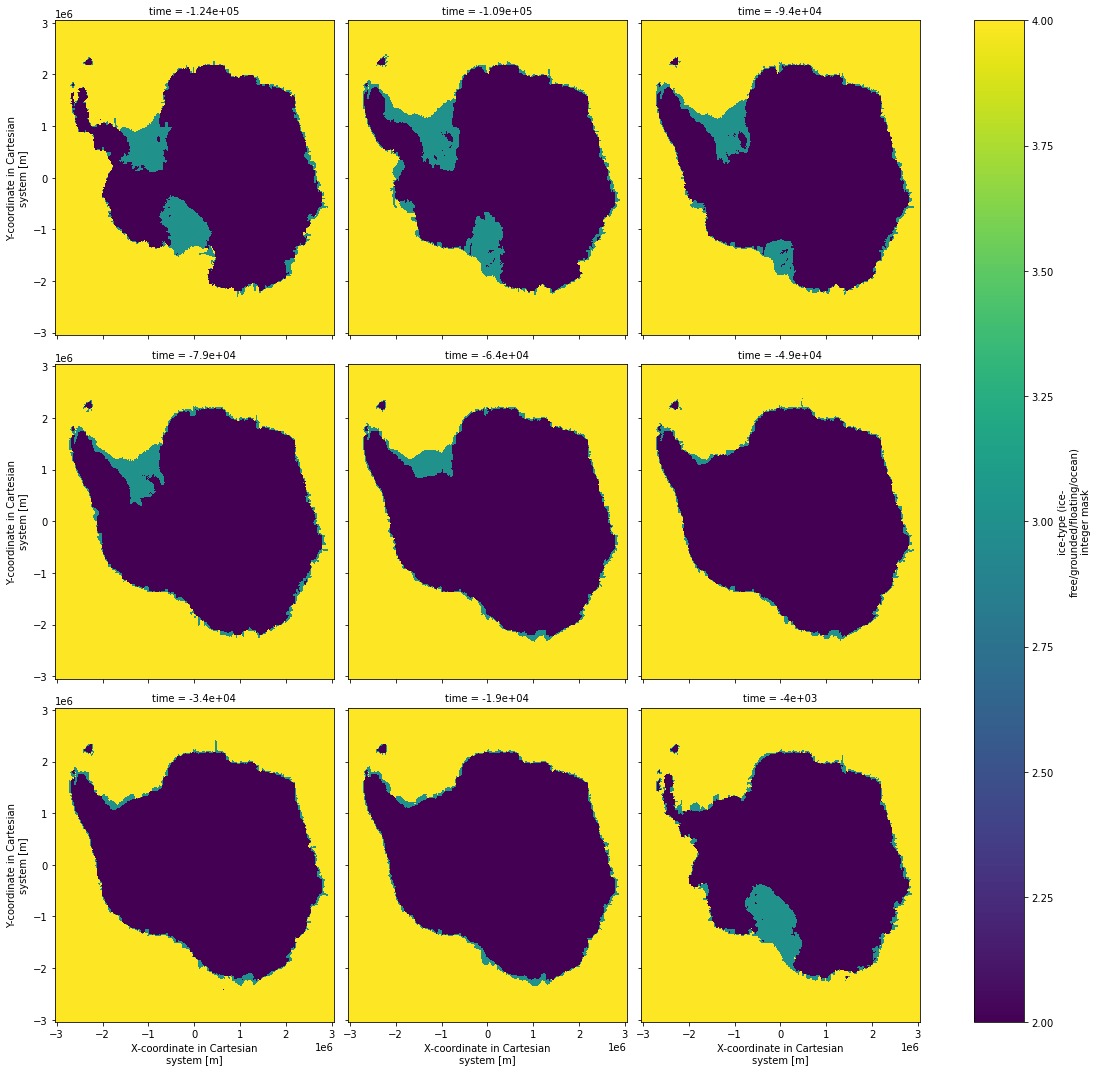
5b. Choose one of the ensemble members and plot masks for several time slices.
[10]:
mask_score_time_series.mask.isel(par_esia=1, par_ppq=2, par_prec=2, par_visc=3,
                       time=slice(0,124,15)).plot(x='x',y='y',col='time',col_wrap=3,size = 5)
[10]:
<xarray.plot.facetgrid.FacetGrid at 0x7f59545ce310>
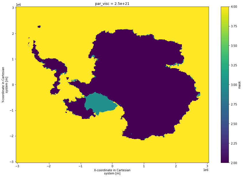
6. Plot a map of the most deglaciated each location becomes across the whole ensemble and all time.
[11]:
mask_score_time_series.mask.isel(par_visc=2).max({"par_esia","par_ppq","par_prec","time"}).plot(size = 10)
[11]:
<matplotlib.collections.QuadMesh at 0x7f59643be2e0>
[ ]: