Intake Tutorial¶

Overview¶

teaching: 20 minutes
exercises: 0
questions:
- How does Intake simplify data discovery, distribution, and loading?

Table of contents¶

Intake primer
Build and intake catalog
Work with an intake catalog
Intake xarray example
Intake STAC example

Intake primer¶

Intake is a lightweight package for finding, investigating, loading and disseminating data. This notebook illutrates the usefulness of intake for a “Data User”. Intake simplifies loading data from many formats into familiar Python objects like Pandas DataFrames or Xarray Datasets. Intake is especially useful for remote datasets - it allows us to bypass downloading data and instead load directly into a Python object for analysis.

Build an intake catalog¶

Let’s say we want to save a version of the data from our geopandas.ipynb tutorial for easy sharing and future use. intake has csv support by default but for loading data with geopandas we need to make sure the intake_geopandas plugin is installed.

[1]:

import intake
import xarray

print(intake.__version__)
xarray.set_options(display_style="html")

0.5.5

[1]:

<xarray.core.options.set_options at 0x7fc3b0606750>

[2]:

# Save data locally from our queries
import pandas as pd
import geopandas as gpd

server = 'https://webservices.volcano.si.edu/geoserver/GVP-VOTW/ows?'
query = 'service=WFS&version=2.0.0&request=GetFeature&typeName=GVP-VOTW:Smithsonian_VOTW_Holocene_Volcanoes&outputFormat=csv'
df = pd.read_csv(server+query)
df.to_csv('votw.csv', index=False)

# Or save as geojson
# Now load query results as json directly in geopandas
query = 'service=WFS&version=2.0.0&request=GetFeature&typeName=GVP-VOTW:Smithsonian_VOTW_Holocene_Volcanoes&outputFormat=json'
gf = gpd.read_file(server+query)
gf.to_file('votw.geojson', driver='GeoJSON')

[3]:

%%writefile votw-intake-catalog.yaml

metadata:
  version: 1

sources:
  votw_pandas:
    args:
      csv_kwargs:
        blocksize: null #prevent reading in parallel with dask
      #urlpath: 'https://webservices.volcano.si.edu/geoserver/GVP-VOTW/ows?service=WFS&version=2.0.0&request=GetFeature&typeName=GVP-VOTW:Smithsonian_VOTW_Holocene_Volcanoes&outputFormat=csv'
      urlpath: './votw.csv'
    description: 'Smithsonian_VOTW_Holocene_Volcanoes 4.8.4'
    driver: csv
    metadata:
      citation: 'Global Volcanism Program, 2013. Volcanoes of the World, v. 4.8.4. Venzke, E (ed.). Smithsonian Institution. Downloaded 06 Dec 2019. https://doi.org/10.5479/si.GVP.VOTW4-2013'
      plots:
        last_eruption_year:
          kind: violin
          by: 'Region'
          y: 'Last_Eruption_Year'
          invert: True
          width: 700
          height: 500


  votw_geopandas:
    args:
      #urlpath: 'https://webservices.volcano.si.edu/geoserver/GVP-VOTW/ows?service=WFS&version=2.0.0&request=GetFeature&typeName=GVP-VOTW:Smithsonian_VOTW_Holocene_Volcanoes&outputFormat=json'
      urlpath: './votw.geojson'
    description: 'Smithsonian_VOTW_Holocene_Volcanoes 4.8.4'
    driver: geojson
    metadata:
      citation: 'Global Volcanism Program, 2013. Volcanoes of the World, v. 4.8.4. Venzke, E (ed.). Smithsonian Institution. Downloaded 06 Dec 2019. https://doi.org/10.5479/si.GVP.VOTW4-2013'

Writing votw-intake-catalog.yaml

[4]:

# put this catalog, votw.csv, and votw.geojson, in a public place like GitHub!
# This facilitates sharing and version controlled analysis
cat = intake.open_catalog('votw-intake-catalog.yaml')

[5]:

print(list(cat))
cat.votw_pandas.description

['votw_pandas', 'votw_geopandas']

[5]:

'Smithsonian_VOTW_Holocene_Volcanoes 4.8.4'

[6]:

# Loading the data is now very straightforward:
# We know the data will be read into a Pandas DataFrame because
cat.votw_pandas.container

[6]:

'dataframe'

[7]:

df = cat.votw_pandas.read()
df.head()

[7]:

	FID	Volcano_Number	Volcano_Name	Primary_Volcano_Type	Last_Eruption_Year	Country	Geological_Summary	Region	Subregion	Latitude	Longitude	Elevation	Tectonic_Setting	Geologic_Epoch	Evidence_Category	Primary_Photo_Link	Primary_Photo_Caption	Primary_Photo_Credit	Major_Rock_Type	GeoLocation
0	Smithsonian_VOTW_Holocene_Volcanoes.fid--71eae...	210010	West Eifel Volcanic Field	Maar(s)	-8300.0	Germany	The West Eifel Volcanic Field of western Germa...	Mediterranean and Western Asia	Western Europe	50.170	6.85	600	Rift zone / Continental crust (> 25 km)	Holocene	Eruption Dated	https://volcano.si.edu/gallery/photos/GVP-0150...	The lake-filled Weinfelder maar is one of abou...	Photo by Richard Waitt, 1990 (U.S. Geological ...	Foidite	POINT (50.17 6.85)
1	Smithsonian_VOTW_Holocene_Volcanoes.fid--71eae...	210020	Chaine des Puys	Lava dome(s)	-4040.0	France	The Chaîne des Puys, prominent in the history ...	Mediterranean and Western Asia	Western Europe	45.775	2.97	1464	Rift zone / Continental crust (> 25 km)	Holocene	Eruption Dated	https://volcano.si.edu/gallery/photos/GVP-0880...	The central part of the Chaîne des Puys volcan...	Photo by Ichio Moriya (Kanazawa University).	Basalt / Picro-Basalt	POINT (45.775 2.97)
2	Smithsonian_VOTW_Holocene_Volcanoes.fid--71eae...	210030	Olot Volcanic Field	Pyroclastic cone(s)	NaN	Spain	The Olot volcanic field (also known as the Gar...	Mediterranean and Western Asia	Western Europe	42.170	2.53	893	Intraplate / Continental crust (> 25 km)	Holocene	Evidence Credible	https://volcano.si.edu/gallery/photos/GVP-1199...	The forested Volcà Montolivet scoria cone rise...	Photo by Puigalder (Wikimedia Commons).	Trachybasalt / Tephrite Basanite	POINT (42.17 2.53)
3	Smithsonian_VOTW_Holocene_Volcanoes.fid--71eae...	210040	Calatrava Volcanic Field	Pyroclastic cone(s)	-3600.0	Spain	The Calatrava volcanic field lies in central S...	Mediterranean and Western Asia	Western Europe	38.870	-4.02	1117	Intraplate / Continental crust (> 25 km)	Holocene	Eruption Dated	https://volcano.si.edu/gallery/photos/GVP-1185...	Columba volcano, the youngest known vent of th...	Photo by Rafael Becerra Ramírez, 2006 (Univers...	Basalt / Picro-Basalt	POINT (38.87 -4.02)
4	Smithsonian_VOTW_Holocene_Volcanoes.fid--71eae...	211003	Vulsini	Caldera	-104.0	Italy	The Vulsini volcanic complex in central Italy ...	Mediterranean and Western Asia	Italy	42.600	11.93	800	Subduction zone / Continental crust (> 25 km)	Holocene	Eruption Observed	https://volcano.si.edu/gallery/photos/GVP-0150...	The 16-km-wide Bolsena caldera containing Lago...	Photo by Richard Waitt, 1985 (U.S. Geological ...	Trachyte / Trachydacite	POINT (42.6 11.93)

[8]:

# Notice we also specified some pre-defined plots in the catalog
# This requires hvplot
import hvplot.pandas
source = cat.votw_pandas
source.plot.last_eruption_year()

[8]:

[9]:

# Load a different dataset in the same catalog
source = cat.votw_geopandas
source.description

[9]:

'Smithsonian_VOTW_Holocene_Volcanoes 4.8.4'

[10]:

gf = source.read()
test = gf.loc[:,['Last_Eruption_Year', 'Volcano_Name', 'geometry']]
test.hvplot.points(geo=True, hover_cols=['Volcano_Name'], color='Last_Eruption_Year')

[10]:

Intake xarray example¶

We’ve seen a plugin to load geospatial vector data into geopandas geodataframes, there is also a plugin to facilitate loading geospatial raster data into xarray dataarrays! https://github.com/intake/intake-xarray

[11]:

# load a catalog stored on github
xcat = intake.open_catalog('https://raw.githubusercontent.com/intake/intake-xarray/master/examples/catalog.yml')
display(list(xcat))

['esgf',
 'geotiff',
 'image',
 'images_labelled',
 'images_unlabelled',
 'grib_thredds']

The use of the intake catalog is much the same as above, except that the data container has switched to xarray objects.

[12]:

geotiff = xcat.geotiff
geotiff.plot.band_image()

[12]:

[13]:

da = geotiff.read()  # to xarray.DataArray
da.max('band')

[13]:

xarray.DataArray

y: 300
x: 300

1.819e+03 2.596e+03 2.495e+03 ... 3.067e+03 3.802e+03 2.665e+03

array([[1819., 2596., 2495., ..., 2429., 1785., 2023.],
       [2259., 2359., 1885., ..., 2158., 1684., 1921.],
       [2865., 2291., 2664., ..., 2302., 2055., 2057.],
       ...,
       [3081., 2679., 2612., ..., 2499., 2098., 1395.],
       [2779., 2544., 2779., ..., 1429., 1596., 1496.],
       [3183., 2309., 2679., ..., 3067., 3802., 2665.]])

Coordinates: (2)

(y)

float64

4.309e+06 4.309e+06 ... 4.264e+06

array([4309200., 4309050., 4308900., ..., 4264650., 4264500., 4264350.])

(x)

float64

3.324e+05 3.326e+05 ... 3.772e+05

array([332400., 332550., 332700., ..., 376950., 377100., 377250.])

Attributes: (0)

Intake STAC example¶

Instead of creating your own metadata catalogs from scratch as YAML files, intake plugins exist to read catalogs in different formats. For example, for geospatial data on the web, SpatioTemporal Asset Catalogs (STAC) are emerging as a standard way to descripe data that you want to search for based on georeference location, time, and perhaps other metadata fields. The intake-stac plugin greatly facilitates loading datasets referenced in STAC catalogs into Python Xarray objects for analysis. https://github.com/pangeo-data/intake-stac

[14]:

stac_cat = intake.open_stac_catalog(
    'https://storage.googleapis.com/pdd-stac/disasters/catalog.json',
    name='planet-disaster-data'
)
display(list(stac_cat))

['20170831_172754_101c',
 '2017831_195552_SS02',
 '20170831_195425_SS02',
 '20170831_162740_ssc1d1',
 'Houston-East-20170831-103f-100d-0f4f-RGB']

[15]:

print(stac_cat['Houston-East-20170831-103f-100d-0f4f-RGB'])

name: Houston-East-20170831-103f-100d-0f4f-RGB
container: catalog
plugin: ['stac_item']
description:
direct_access: True
user_parameters: []
metadata:
args:
  stac_obj: Houston-East-20170831-103f-100d-0f4f-RGB

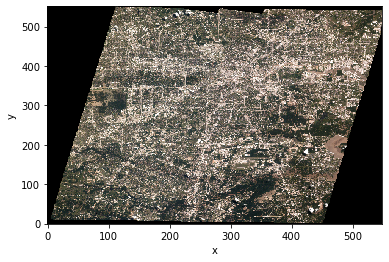
Entries in the catalog are accessed just like above. Below we pull the thumbnail image from the Hurricane Harvey composite image.

[16]:

da = stac_cat['Houston-East-20170831-103f-100d-0f4f-RGB']['thumbnail'].to_dask()
da

[16]: