
Xarray Tutorial
Overview
teaching: 30 minutes
exercises: 0
questions:
What is xarray designed to do?
How do I create an xarray Dataset?
How does indexing work with xarray?
How do I run computations on xarray datasets?
What are ways to ploy xarray datasets?
Table of contents
Xarray primer
We’ve seen that Pandas and Geopandas are excellent libraries for analyzing tabular “labeled data”. Xarray is designed to make it easier to work with with labeled multidimensional data. By multidimensional data (also often called N-dimensional), we mean data with many independent dimensions or axes. For example, we might represent Earth’s surface temperature \(T\) as a three dimensional variable
where \(x\) and \(y\) are spatial dimensions and and \(t\) is time. By labeled, we mean data that has metadata associated with it describing the names and relationships between the variables. The cartoon below shows a “data cube” schematic dataset with temperature and preciptation sharing the same three dimensions, plus longitude and latitude as auxilliary coordinates.

Xarray data structures
Like Pandas, xarray has two fundamental data structures: * a DataArray, which holds a single multi-dimensional variable and its coordinates * a Dataset, which holds multiple variables that potentially share the same coordinates
A DataArray has four essential attributes: * values: a numpy.ndarray holding the array’s values * dims: dimension names for each axis (e.g., ('x', 'y', 'z')) * coords: a dict-like container of arrays (coordinates) that label each point (e.g., 1-dimensional arrays of numbers, datetime objects or strings) * attrs: an OrderedDict to hold arbitrary metadata (attributes)
A dataset is simply an object containing multiple DataArrays indexed by variable name
Creating data
Let’s start by constructing some DataArrays manually
[1]:
import numpy as np
import xarray as xr
[2]:
print('Numpy version: ', np.__version__)
print('Xarray version: ', xr.__version__)
Numpy version:  1.18.4
Xarray version:  0.15.1
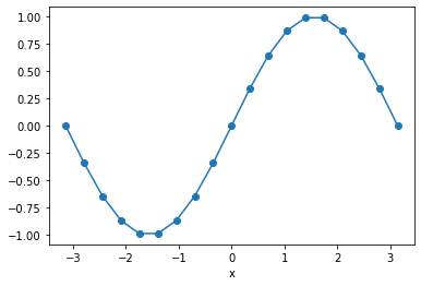
Here we model the simple function
on the interval \(-\pi\) to \(\pi\). We start by creating the data as numpy arrays.
[3]:
x = np.linspace(-np.pi, np.pi, 19)
f = np.sin(x)
Now we are going to put this into an xarray DataArray.
A simple DataArray without dimensions or coordinates isn’t much use.
[4]:
da_f = xr.DataArray(f)
da_f
[4]:
- dim_0: 19
- -1.225e-16 -0.342 -0.6428 -0.866 ... 0.866 0.6428 0.342 1.225e-16
array([-1.22464680e-16, -3.42020143e-01, -6.42787610e-01, -8.66025404e-01,
       -9.84807753e-01, -9.84807753e-01, -8.66025404e-01, -6.42787610e-01,
       -3.42020143e-01,  0.00000000e+00,  3.42020143e-01,  6.42787610e-01,
        8.66025404e-01,  9.84807753e-01,  9.84807753e-01,  8.66025404e-01,
        6.42787610e-01,  3.42020143e-01,  1.22464680e-16])
We can add a dimension name…
[5]:
da_f = xr.DataArray(f, dims=['x'])
da_f
[5]:
- x: 19
- -1.225e-16 -0.342 -0.6428 -0.866 ... 0.866 0.6428 0.342 1.225e-16
array([-1.22464680e-16, -3.42020143e-01, -6.42787610e-01, -8.66025404e-01,
       -9.84807753e-01, -9.84807753e-01, -8.66025404e-01, -6.42787610e-01,
       -3.42020143e-01,  0.00000000e+00,  3.42020143e-01,  6.42787610e-01,
        8.66025404e-01,  9.84807753e-01,  9.84807753e-01,  8.66025404e-01,
        6.42787610e-01,  3.42020143e-01,  1.22464680e-16])
But things get most interesting when we add a coordinate:
[6]:
da_f = xr.DataArray(f, dims=['x'], coords={'x': x})
da_f
[6]:
- x: 19
- -1.225e-16 -0.342 -0.6428 -0.866 ... 0.866 0.6428 0.342 1.225e-16
array([-1.22464680e-16, -3.42020143e-01, -6.42787610e-01, -8.66025404e-01, -9.84807753e-01, -9.84807753e-01, -8.66025404e-01, -6.42787610e-01, -3.42020143e-01, 0.00000000e+00, 3.42020143e-01, 6.42787610e-01, 8.66025404e-01, 9.84807753e-01, 9.84807753e-01, 8.66025404e-01, 6.42787610e-01, 3.42020143e-01, 1.22464680e-16]) - x(x)float64-3.142 -2.793 ... 2.793 3.142
array([-3.141593, -2.792527, -2.443461, -2.094395, -1.745329, -1.396263,
       -1.047198, -0.698132, -0.349066,  0.      ,  0.349066,  0.698132,
        1.047198,  1.396263,  1.745329,  2.094395,  2.443461,  2.792527,
        3.141593])
Xarray has built-in plotting, like pandas.
[7]:
da_f.plot(marker='o')
[7]:
[<matplotlib.lines.Line2D at 0x7fc69bff1990>]
Selecting Data
We can always use regular numpy indexing and slicing on DataArrays to get the data back out.
[8]:
# get the 10th item
da_f[10]
[8]:
- 0.342
array(0.34202014)
- x()float640.3491
array(0.34906585)
[9]:
# get the first 10 items
da_f[:10]
[9]:
- x: 10
- -1.225e-16 -0.342 -0.6428 -0.866 -0.9848 ... -0.866 -0.6428 -0.342 0.0
array([-1.22464680e-16, -3.42020143e-01, -6.42787610e-01, -8.66025404e-01, -9.84807753e-01, -9.84807753e-01, -8.66025404e-01, -6.42787610e-01, -3.42020143e-01, 0.00000000e+00]) - x(x)float64-3.142 -2.793 ... -0.3491 0.0
array([-3.141593, -2.792527, -2.443461, -2.094395, -1.745329, -1.396263,
       -1.047198, -0.698132, -0.349066,  0.      ])
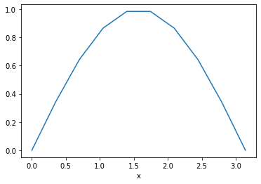
However, it is often much more powerful to use xarray’s .sel() method to use label-based indexing. This allows us to fetch values based on the value of the coordinate, not the numerical index.
[10]:
da_f.sel(x=0)
[10]:
- 0.0
array(0.)
- x()float640.0
array(0.)
[11]:
da_f.sel(x=slice(0, np.pi)).plot()
[11]:
[<matplotlib.lines.Line2D at 0x7fc69be70f10>]
Basic Computations
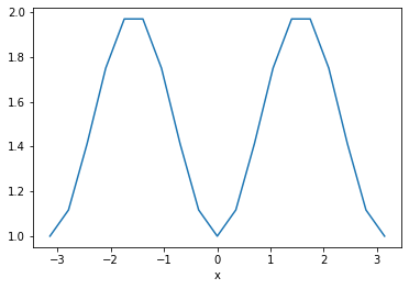
When we perform mathematical manipulations of xarray DataArrays, the coordinates come along for the ride. Imagine we want to calcuate
We can apply familiar numpy operations to xarray objects.
[12]:
da_g = da_f**2 + 1
da_g
[12]:
- x: 19
- 1.0 1.117 1.413 1.75 1.97 1.97 1.75 ... 1.97 1.97 1.75 1.413 1.117 1.0
array([1. , 1.11697778, 1.41317591, 1.75 , 1.96984631, 1.96984631, 1.75 , 1.41317591, 1.11697778, 1. , 1.11697778, 1.41317591, 1.75 , 1.96984631, 1.96984631, 1.75 , 1.41317591, 1.11697778, 1. ]) - x(x)float64-3.142 -2.793 ... 2.793 3.142
array([-3.141593, -2.792527, -2.443461, -2.094395, -1.745329, -1.396263,
       -1.047198, -0.698132, -0.349066,  0.      ,  0.349066,  0.698132,
        1.047198,  1.396263,  1.745329,  2.094395,  2.443461,  2.792527,
        3.141593])
[13]:
da_g.plot()
[13]:
[<matplotlib.lines.Line2D at 0x7fc69bde8cd0>]
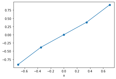
Exercise
Multipy the DataArrays
da_fandda_gtogether.Select the range \(-1 < x < 1\)
Plot the result
[14]:
(da_f * da_g).sel(x=slice(-1, 1)).plot(marker='o')
[14]:
[<matplotlib.lines.Line2D at 0x7fc69bd5a590>]
Multidimensional Data
If we are just dealing with 1D data, Pandas and Xarray have very similar capabilities. Xarray’s real potential comes with multidimensional data.
At this point we will load data from a netCDF file into an xarray dataset.
[15]:
%%bash

git clone https://github.com/pangeo-data/tutorial-data.git
Cloning into 'tutorial-data'...
[16]:
ds = xr.open_dataset('./tutorial-data/sst/NOAA_NCDC_ERSST_v3b_SST-1960.nc')
ds
[16]:
- lat: 89
- lon: 180
- time: 12
- lat(lat)float32-88.0 -86.0 -84.0 ... 86.0 88.0
- standard_name :
- latitude
- pointwidth :
- 2.0
- gridtype :
- 0
- units :
- degree_north
array([-88., -86., -84., -82., -80., -78., -76., -74., -72., -70., -68., -66., -64., -62., -60., -58., -56., -54., -52., -50., -48., -46., -44., -42., -40., -38., -36., -34., -32., -30., -28., -26., -24., -22., -20., -18., -16., -14., -12., -10., -8., -6., -4., -2., 0., 2., 4., 6., 8., 10., 12., 14., 16., 18., 20., 22., 24., 26., 28., 30., 32., 34., 36., 38., 40., 42., 44., 46., 48., 50., 52., 54., 56., 58., 60., 62., 64., 66., 68., 70., 72., 74., 76., 78., 80., 82., 84., 86., 88.], dtype=float32) - lon(lon)float320.0 2.0 4.0 ... 354.0 356.0 358.0
- standard_name :
- longitude
- pointwidth :
- 2.0
- gridtype :
- 1
- units :
- degree_east
array([ 0., 2., 4., 6., 8., 10., 12., 14., 16., 18., 20., 22., 24., 26., 28., 30., 32., 34., 36., 38., 40., 42., 44., 46., 48., 50., 52., 54., 56., 58., 60., 62., 64., 66., 68., 70., 72., 74., 76., 78., 80., 82., 84., 86., 88., 90., 92., 94., 96., 98., 100., 102., 104., 106., 108., 110., 112., 114., 116., 118., 120., 122., 124., 126., 128., 130., 132., 134., 136., 138., 140., 142., 144., 146., 148., 150., 152., 154., 156., 158., 160., 162., 164., 166., 168., 170., 172., 174., 176., 178., 180., 182., 184., 186., 188., 190., 192., 194., 196., 198., 200., 202., 204., 206., 208., 210., 212., 214., 216., 218., 220., 222., 224., 226., 228., 230., 232., 234., 236., 238., 240., 242., 244., 246., 248., 250., 252., 254., 256., 258., 260., 262., 264., 266., 268., 270., 272., 274., 276., 278., 280., 282., 284., 286., 288., 290., 292., 294., 296., 298., 300., 302., 304., 306., 308., 310., 312., 314., 316., 318., 320., 322., 324., 326., 328., 330., 332., 334., 336., 338., 340., 342., 344., 346., 348., 350., 352., 354., 356., 358.], dtype=float32) - time(time)datetime64[ns]1960-01-15 ... 1960-12-15
array(['1960-01-15T00:00:00.000000000', '1960-02-15T00:00:00.000000000',
       '1960-03-15T00:00:00.000000000', '1960-04-15T00:00:00.000000000',
       '1960-05-15T00:00:00.000000000', '1960-06-15T00:00:00.000000000',
       '1960-07-15T00:00:00.000000000', '1960-08-15T00:00:00.000000000',
       '1960-09-15T00:00:00.000000000', '1960-10-15T00:00:00.000000000',
       '1960-11-15T00:00:00.000000000', '1960-12-15T00:00:00.000000000'],
      dtype='datetime64[ns]')
- sst(time, lat, lon)float32...
- pointwidth :
- 1.0
- valid_min :
- -3.0
- valid_max :
- 45.0
- units :
- degree_Celsius
- long_name :
- Extended reconstructed sea surface temperature
- standard_name :
- sea_surface_temperature
- iridl:hasSemantics :
- iridl:SeaSurfaceTemperature
[192240 values with dtype=float32]
- Conventions :
- IRIDL
- source :
- https://iridl.ldeo.columbia.edu/SOURCES/.NOAA/.NCDC/.ERSST/.version3b/.sst/
- history :
- extracted and cleaned by Ryan Abernathey for Research Computing in Earth Science
[17]:
## Xarray > v0.14.1 has a new HTML output type!
xr.set_options(display_style="html")
ds
[17]:
- lat: 89
- lon: 180
- time: 12
- lat(lat)float32-88.0 -86.0 -84.0 ... 86.0 88.0
- standard_name :
- latitude
- pointwidth :
- 2.0
- gridtype :
- 0
- units :
- degree_north
array([-88., -86., -84., -82., -80., -78., -76., -74., -72., -70., -68., -66., -64., -62., -60., -58., -56., -54., -52., -50., -48., -46., -44., -42., -40., -38., -36., -34., -32., -30., -28., -26., -24., -22., -20., -18., -16., -14., -12., -10., -8., -6., -4., -2., 0., 2., 4., 6., 8., 10., 12., 14., 16., 18., 20., 22., 24., 26., 28., 30., 32., 34., 36., 38., 40., 42., 44., 46., 48., 50., 52., 54., 56., 58., 60., 62., 64., 66., 68., 70., 72., 74., 76., 78., 80., 82., 84., 86., 88.], dtype=float32) - lon(lon)float320.0 2.0 4.0 ... 354.0 356.0 358.0
- standard_name :
- longitude
- pointwidth :
- 2.0
- gridtype :
- 1
- units :
- degree_east
array([ 0., 2., 4., 6., 8., 10., 12., 14., 16., 18., 20., 22., 24., 26., 28., 30., 32., 34., 36., 38., 40., 42., 44., 46., 48., 50., 52., 54., 56., 58., 60., 62., 64., 66., 68., 70., 72., 74., 76., 78., 80., 82., 84., 86., 88., 90., 92., 94., 96., 98., 100., 102., 104., 106., 108., 110., 112., 114., 116., 118., 120., 122., 124., 126., 128., 130., 132., 134., 136., 138., 140., 142., 144., 146., 148., 150., 152., 154., 156., 158., 160., 162., 164., 166., 168., 170., 172., 174., 176., 178., 180., 182., 184., 186., 188., 190., 192., 194., 196., 198., 200., 202., 204., 206., 208., 210., 212., 214., 216., 218., 220., 222., 224., 226., 228., 230., 232., 234., 236., 238., 240., 242., 244., 246., 248., 250., 252., 254., 256., 258., 260., 262., 264., 266., 268., 270., 272., 274., 276., 278., 280., 282., 284., 286., 288., 290., 292., 294., 296., 298., 300., 302., 304., 306., 308., 310., 312., 314., 316., 318., 320., 322., 324., 326., 328., 330., 332., 334., 336., 338., 340., 342., 344., 346., 348., 350., 352., 354., 356., 358.], dtype=float32) - time(time)datetime64[ns]1960-01-15 ... 1960-12-15
array(['1960-01-15T00:00:00.000000000', '1960-02-15T00:00:00.000000000',
       '1960-03-15T00:00:00.000000000', '1960-04-15T00:00:00.000000000',
       '1960-05-15T00:00:00.000000000', '1960-06-15T00:00:00.000000000',
       '1960-07-15T00:00:00.000000000', '1960-08-15T00:00:00.000000000',
       '1960-09-15T00:00:00.000000000', '1960-10-15T00:00:00.000000000',
       '1960-11-15T00:00:00.000000000', '1960-12-15T00:00:00.000000000'],
      dtype='datetime64[ns]')
- sst(time, lat, lon)float32...
- pointwidth :
- 1.0
- valid_min :
- -3.0
- valid_max :
- 45.0
- units :
- degree_Celsius
- long_name :
- Extended reconstructed sea surface temperature
- standard_name :
- sea_surface_temperature
- iridl:hasSemantics :
- iridl:SeaSurfaceTemperature
[192240 values with dtype=float32]
- Conventions :
- IRIDL
- source :
- https://iridl.ldeo.columbia.edu/SOURCES/.NOAA/.NCDC/.ERSST/.version3b/.sst/
- history :
- extracted and cleaned by Ryan Abernathey for Research Computing in Earth Science
[18]:
# both do the exact same thing

# dictionary syntax
sst = ds['sst']

# attribute syntax
sst = ds.sst

sst
[18]:
- time: 12
- lat: 89
- lon: 180
- ...
[192240 values with dtype=float32]
- lat(lat)float32-88.0 -86.0 -84.0 ... 86.0 88.0
- standard_name :
- latitude
- pointwidth :
- 2.0
- gridtype :
- 0
- units :
- degree_north
array([-88., -86., -84., -82., -80., -78., -76., -74., -72., -70., -68., -66., -64., -62., -60., -58., -56., -54., -52., -50., -48., -46., -44., -42., -40., -38., -36., -34., -32., -30., -28., -26., -24., -22., -20., -18., -16., -14., -12., -10., -8., -6., -4., -2., 0., 2., 4., 6., 8., 10., 12., 14., 16., 18., 20., 22., 24., 26., 28., 30., 32., 34., 36., 38., 40., 42., 44., 46., 48., 50., 52., 54., 56., 58., 60., 62., 64., 66., 68., 70., 72., 74., 76., 78., 80., 82., 84., 86., 88.], dtype=float32) - lon(lon)float320.0 2.0 4.0 ... 354.0 356.0 358.0
- standard_name :
- longitude
- pointwidth :
- 2.0
- gridtype :
- 1
- units :
- degree_east
array([ 0., 2., 4., 6., 8., 10., 12., 14., 16., 18., 20., 22., 24., 26., 28., 30., 32., 34., 36., 38., 40., 42., 44., 46., 48., 50., 52., 54., 56., 58., 60., 62., 64., 66., 68., 70., 72., 74., 76., 78., 80., 82., 84., 86., 88., 90., 92., 94., 96., 98., 100., 102., 104., 106., 108., 110., 112., 114., 116., 118., 120., 122., 124., 126., 128., 130., 132., 134., 136., 138., 140., 142., 144., 146., 148., 150., 152., 154., 156., 158., 160., 162., 164., 166., 168., 170., 172., 174., 176., 178., 180., 182., 184., 186., 188., 190., 192., 194., 196., 198., 200., 202., 204., 206., 208., 210., 212., 214., 216., 218., 220., 222., 224., 226., 228., 230., 232., 234., 236., 238., 240., 242., 244., 246., 248., 250., 252., 254., 256., 258., 260., 262., 264., 266., 268., 270., 272., 274., 276., 278., 280., 282., 284., 286., 288., 290., 292., 294., 296., 298., 300., 302., 304., 306., 308., 310., 312., 314., 316., 318., 320., 322., 324., 326., 328., 330., 332., 334., 336., 338., 340., 342., 344., 346., 348., 350., 352., 354., 356., 358.], dtype=float32) - time(time)datetime64[ns]1960-01-15 ... 1960-12-15
array(['1960-01-15T00:00:00.000000000', '1960-02-15T00:00:00.000000000',
       '1960-03-15T00:00:00.000000000', '1960-04-15T00:00:00.000000000',
       '1960-05-15T00:00:00.000000000', '1960-06-15T00:00:00.000000000',
       '1960-07-15T00:00:00.000000000', '1960-08-15T00:00:00.000000000',
       '1960-09-15T00:00:00.000000000', '1960-10-15T00:00:00.000000000',
       '1960-11-15T00:00:00.000000000', '1960-12-15T00:00:00.000000000'],
      dtype='datetime64[ns]')
- pointwidth :
- 1.0
- valid_min :
- -3.0
- valid_max :
- 45.0
- units :
- degree_Celsius
- long_name :
- Extended reconstructed sea surface temperature
- standard_name :
- sea_surface_temperature
- iridl:hasSemantics :
- iridl:SeaSurfaceTemperature
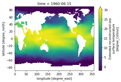
Multidimensional Indexing
In this example, we take advantage of the fact that xarray understands time to select a particular date
[19]:
sst.sel(time='1960-06-15').plot(vmin=-2, vmax=30)
[19]:
<matplotlib.collections.QuadMesh at 0x7fc69b0ffd10>
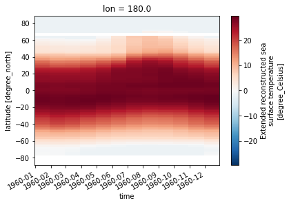
But we can select along any axis
[20]:
sst.sel(lon=180).transpose().plot()
[20]:
<matplotlib.collections.QuadMesh at 0x7fc69b0c9ed0>
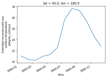
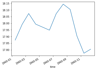
[21]:
sst.sel(lon=180, lat=40).plot()
[21]:
[<matplotlib.lines.Line2D at 0x7fc69af6c250>]
Label-Based Reduction Operations
Usually the process of data analysis involves going from a big, multidimensional dataset to a few concise figures. Inevitably, the data must be “reduced” somehow. Examples of simple reduction operations include:
Mean
Standard Deviation
Minimum
Maximum
etc. Xarray supports all of these and more, via a familiar numpy-like syntax. But with xarray, you can specify the reductions by dimension.
First we start with the default, reduction over all dimensions:
[22]:
sst.mean()
[22]:
- 13.626506
array(13.626506, dtype=float32)
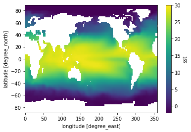
[23]:
sst_time_mean = sst.mean(dim='time')
sst_time_mean.plot(vmin=-2, vmax=30)
/srv/conda/envs/notebook/lib/python3.7/site-packages/xarray/core/nanops.py:142: RuntimeWarning: Mean of empty slice
  return np.nanmean(a, axis=axis, dtype=dtype)
[23]:
<matplotlib.collections.QuadMesh at 0x7fc69ae94f10>
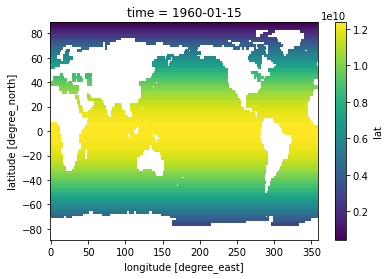
[24]:
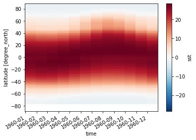
sst_zonal_mean = sst.mean(dim='lon')
sst_zonal_mean.transpose().plot()
[24]:
<matplotlib.collections.QuadMesh at 0x7fc69aee1050>
[25]:
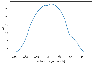
sst_time_and_zonal_mean = sst.mean(dim=('time', 'lon'))
sst_time_and_zonal_mean.plot()
[25]:
[<matplotlib.lines.Line2D at 0x7fc69be2a150>]
[26]:
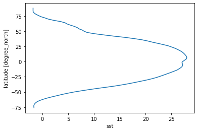
# some might prefer to have lat on the y axis
sst_time_and_zonal_mean.plot(y='lat')
[26]:
[<matplotlib.lines.Line2D at 0x7fc69aee1fd0>]
More Complicated Example: Weighted Mean
The means we calculated above were “naive”; they were straightforward numerical means over the different dimensions of the dataset. They did not account, for example, for spherical geometry of the globe and the necessary weighting factors. Although xarray is very useful for geospatial analysis, it has no built-in understanding of geography.
Below we show how to create a proper weighted mean by using the formula for the area element in spherical coordinates. This is a good illustration of several xarray concepts.
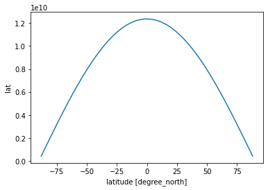
The area element for lat-lon coordinates is
where \(\phi\) is latitude, \(\delta \phi\) is the spacing of the points in latitude, \(\delta \lambda\) is the spacing of the points in longitude, and \(R\) is Earth’s radius. (In this formula, \(\phi\) and \(\lambda\) are measured in radians.) Let’s use xarray to create the weight factor.
[27]:
R = 6.37e6
# we know already that the spacing of the points is one degree latitude
dϕ = np.deg2rad(1.)
dλ = np.deg2rad(1.)
dA = R**2 * dϕ * dλ * np.cos(np.deg2rad(ds.lat))
dA.plot()
[27]:
[<matplotlib.lines.Line2D at 0x7fc69ac60cd0>]
[28]:
dA.where(sst[0].notnull())
[28]:
- lat: 89
- lon: 180
- nan nan nan nan ... 431372740.0 431372740.0 431372740.0 431372740.0
array([[ nan, nan, nan, ..., nan, nan, nan], [ nan, nan, nan, ..., nan, nan, nan], [ nan, nan, nan, ..., nan, nan, nan], ..., [1.2920163e+09, 1.2920163e+09, 1.2920163e+09, ..., 1.2920163e+09, 1.2920163e+09, 1.2920163e+09], [8.6222048e+08, 8.6222048e+08, 8.6222048e+08, ..., 8.6222048e+08, 8.6222048e+08, 8.6222048e+08], [4.3137274e+08, 4.3137274e+08, 4.3137274e+08, ..., 4.3137274e+08, 4.3137274e+08, 4.3137274e+08]], dtype=float32) - lat(lat)float32-88.0 -86.0 -84.0 ... 86.0 88.0
- standard_name :
- latitude
- pointwidth :
- 2.0
- gridtype :
- 0
- units :
- degree_north
array([-88., -86., -84., -82., -80., -78., -76., -74., -72., -70., -68., -66., -64., -62., -60., -58., -56., -54., -52., -50., -48., -46., -44., -42., -40., -38., -36., -34., -32., -30., -28., -26., -24., -22., -20., -18., -16., -14., -12., -10., -8., -6., -4., -2., 0., 2., 4., 6., 8., 10., 12., 14., 16., 18., 20., 22., 24., 26., 28., 30., 32., 34., 36., 38., 40., 42., 44., 46., 48., 50., 52., 54., 56., 58., 60., 62., 64., 66., 68., 70., 72., 74., 76., 78., 80., 82., 84., 86., 88.], dtype=float32) - lon(lon)float320.0 2.0 4.0 ... 354.0 356.0 358.0
- standard_name :
- longitude
- pointwidth :
- 2.0
- gridtype :
- 1
- units :
- degree_east
array([ 0., 2., 4., 6., 8., 10., 12., 14., 16., 18., 20., 22., 24., 26., 28., 30., 32., 34., 36., 38., 40., 42., 44., 46., 48., 50., 52., 54., 56., 58., 60., 62., 64., 66., 68., 70., 72., 74., 76., 78., 80., 82., 84., 86., 88., 90., 92., 94., 96., 98., 100., 102., 104., 106., 108., 110., 112., 114., 116., 118., 120., 122., 124., 126., 128., 130., 132., 134., 136., 138., 140., 142., 144., 146., 148., 150., 152., 154., 156., 158., 160., 162., 164., 166., 168., 170., 172., 174., 176., 178., 180., 182., 184., 186., 188., 190., 192., 194., 196., 198., 200., 202., 204., 206., 208., 210., 212., 214., 216., 218., 220., 222., 224., 226., 228., 230., 232., 234., 236., 238., 240., 242., 244., 246., 248., 250., 252., 254., 256., 258., 260., 262., 264., 266., 268., 270., 272., 274., 276., 278., 280., 282., 284., 286., 288., 290., 292., 294., 296., 298., 300., 302., 304., 306., 308., 310., 312., 314., 316., 318., 320., 322., 324., 326., 328., 330., 332., 334., 336., 338., 340., 342., 344., 346., 348., 350., 352., 354., 356., 358.], dtype=float32) - time()datetime64[ns]1960-01-15
array('1960-01-15T00:00:00.000000000', dtype='datetime64[ns]')
[29]:
pixel_area = dA.where(sst[0].notnull())
pixel_area.plot()
[29]:
<matplotlib.collections.QuadMesh at 0x7fc69ac23190>
[30]:
total_ocean_area = pixel_area.sum(dim=('lon', 'lat'))
sst_weighted_mean = (sst * pixel_area).sum(dim=('lon', 'lat')) / total_ocean_area
sst_weighted_mean.plot()
[30]:
[<matplotlib.lines.Line2D at 0x7fc69ad11150>]
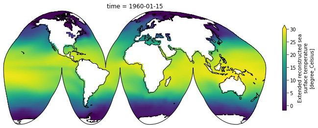
Maps
Xarray integrates with cartopy to enable you to plot your data on a map
[31]:
import matplotlib.pyplot as plt
import cartopy.crs as ccrs

plt.figure(figsize=(12, 8))
ax = plt.axes(projection=ccrs.InterruptedGoodeHomolosine())
ax.coastlines()

sst[0].plot(transform=ccrs.PlateCarree(), vmin=-2, vmax=30,
            cbar_kwargs={'shrink': 0.4})
[31]:
<matplotlib.collections.QuadMesh at 0x7fc6949a3f90>
/srv/conda/envs/notebook/lib/python3.7/site-packages/cartopy/io/__init__.py:260: DownloadWarning: Downloading: http://naciscdn.org/naturalearth/110m/physical/ne_110m_coastline.zip
  warnings.warn('Downloading: {}'.format(url), DownloadWarning)
IV. Opening Many Files
One of the killer features of xarray is its ability to open many files into a single dataset. We do this with the open_mfdataset function.
[32]:
ds_all = xr.open_mfdataset('./tutorial-data/sst/*nc', combine='by_coords')
ds_all
[32]:
- lat: 89
- lon: 180
- time: 684
- lon(lon)float320.0 2.0 4.0 ... 354.0 356.0 358.0
- standard_name :
- longitude
- pointwidth :
- 2.0
- gridtype :
- 1
- units :
- degree_east
array([ 0., 2., 4., 6., 8., 10., 12., 14., 16., 18., 20., 22., 24., 26., 28., 30., 32., 34., 36., 38., 40., 42., 44., 46., 48., 50., 52., 54., 56., 58., 60., 62., 64., 66., 68., 70., 72., 74., 76., 78., 80., 82., 84., 86., 88., 90., 92., 94., 96., 98., 100., 102., 104., 106., 108., 110., 112., 114., 116., 118., 120., 122., 124., 126., 128., 130., 132., 134., 136., 138., 140., 142., 144., 146., 148., 150., 152., 154., 156., 158., 160., 162., 164., 166., 168., 170., 172., 174., 176., 178., 180., 182., 184., 186., 188., 190., 192., 194., 196., 198., 200., 202., 204., 206., 208., 210., 212., 214., 216., 218., 220., 222., 224., 226., 228., 230., 232., 234., 236., 238., 240., 242., 244., 246., 248., 250., 252., 254., 256., 258., 260., 262., 264., 266., 268., 270., 272., 274., 276., 278., 280., 282., 284., 286., 288., 290., 292., 294., 296., 298., 300., 302., 304., 306., 308., 310., 312., 314., 316., 318., 320., 322., 324., 326., 328., 330., 332., 334., 336., 338., 340., 342., 344., 346., 348., 350., 352., 354., 356., 358.], dtype=float32) - lat(lat)float32-88.0 -86.0 -84.0 ... 86.0 88.0
- standard_name :
- latitude
- pointwidth :
- 2.0
- gridtype :
- 0
- units :
- degree_north
array([-88., -86., -84., -82., -80., -78., -76., -74., -72., -70., -68., -66., -64., -62., -60., -58., -56., -54., -52., -50., -48., -46., -44., -42., -40., -38., -36., -34., -32., -30., -28., -26., -24., -22., -20., -18., -16., -14., -12., -10., -8., -6., -4., -2., 0., 2., 4., 6., 8., 10., 12., 14., 16., 18., 20., 22., 24., 26., 28., 30., 32., 34., 36., 38., 40., 42., 44., 46., 48., 50., 52., 54., 56., 58., 60., 62., 64., 66., 68., 70., 72., 74., 76., 78., 80., 82., 84., 86., 88.], dtype=float32) - time(time)datetime64[ns]1960-01-15 ... 2016-12-15
array(['1960-01-15T00:00:00.000000000', '1960-02-15T00:00:00.000000000',
       '1960-03-15T00:00:00.000000000', ..., '2016-10-15T00:00:00.000000000',
       '2016-11-15T00:00:00.000000000', '2016-12-15T00:00:00.000000000'],
      dtype='datetime64[ns]')
- sst(time, lat, lon)float32dask.array<chunksize=(12, 89, 180), meta=np.ndarray>
- pointwidth :
- 1.0
- valid_min :
- -3.0
- valid_max :
- 45.0
- units :
- degree_Celsius
- long_name :
- Extended reconstructed sea surface temperature
- standard_name :
- sea_surface_temperature
- iridl:hasSemantics :
- iridl:SeaSurfaceTemperature
Array Chunk Bytes 43.83 MB 768.96 kB Shape (684, 89, 180) (12, 89, 180) Count 171 Tasks 57 Chunks Type float32 numpy.ndarray
- Conventions :
- IRIDL
- source :
- https://iridl.ldeo.columbia.edu/SOURCES/.NOAA/.NCDC/.ERSST/.version3b/.sst/
- history :
- extracted and cleaned by Ryan Abernathey for Research Computing in Earth Science
Now we have 57 years of data instead of one!
V. Groupby
Now that we have a bigger dataset, this is a good time to check out xarray’s groupby capabilities.
[33]:
sst_clim = ds_all.sst.groupby('time.month').mean(dim='time')
sst_clim
[33]:
- month: 12
- lat: 89
- lon: 180
- dask.array<chunksize=(1, 89, 180), meta=np.ndarray>
Array Chunk Bytes 768.96 kB 64.08 kB Shape (12, 89, 180) (1, 89, 180) Count 1791 Tasks 12 Chunks Type float32 numpy.ndarray - lon(lon)float320.0 2.0 4.0 ... 354.0 356.0 358.0
- standard_name :
- longitude
- pointwidth :
- 2.0
- gridtype :
- 1
- units :
- degree_east
array([ 0., 2., 4., 6., 8., 10., 12., 14., 16., 18., 20., 22., 24., 26., 28., 30., 32., 34., 36., 38., 40., 42., 44., 46., 48., 50., 52., 54., 56., 58., 60., 62., 64., 66., 68., 70., 72., 74., 76., 78., 80., 82., 84., 86., 88., 90., 92., 94., 96., 98., 100., 102., 104., 106., 108., 110., 112., 114., 116., 118., 120., 122., 124., 126., 128., 130., 132., 134., 136., 138., 140., 142., 144., 146., 148., 150., 152., 154., 156., 158., 160., 162., 164., 166., 168., 170., 172., 174., 176., 178., 180., 182., 184., 186., 188., 190., 192., 194., 196., 198., 200., 202., 204., 206., 208., 210., 212., 214., 216., 218., 220., 222., 224., 226., 228., 230., 232., 234., 236., 238., 240., 242., 244., 246., 248., 250., 252., 254., 256., 258., 260., 262., 264., 266., 268., 270., 272., 274., 276., 278., 280., 282., 284., 286., 288., 290., 292., 294., 296., 298., 300., 302., 304., 306., 308., 310., 312., 314., 316., 318., 320., 322., 324., 326., 328., 330., 332., 334., 336., 338., 340., 342., 344., 346., 348., 350., 352., 354., 356., 358.], dtype=float32) - lat(lat)float32-88.0 -86.0 -84.0 ... 86.0 88.0
- standard_name :
- latitude
- pointwidth :
- 2.0
- gridtype :
- 0
- units :
- degree_north
array([-88., -86., -84., -82., -80., -78., -76., -74., -72., -70., -68., -66., -64., -62., -60., -58., -56., -54., -52., -50., -48., -46., -44., -42., -40., -38., -36., -34., -32., -30., -28., -26., -24., -22., -20., -18., -16., -14., -12., -10., -8., -6., -4., -2., 0., 2., 4., 6., 8., 10., 12., 14., 16., 18., 20., 22., 24., 26., 28., 30., 32., 34., 36., 38., 40., 42., 44., 46., 48., 50., 52., 54., 56., 58., 60., 62., 64., 66., 68., 70., 72., 74., 76., 78., 80., 82., 84., 86., 88.], dtype=float32) - month(month)int641 2 3 4 5 6 7 8 9 10 11 12
array([ 1, 2, 3, 4, 5, 6, 7, 8, 9, 10, 11, 12])
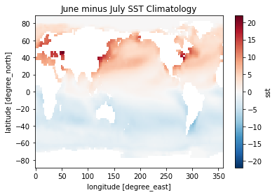
Now the data has dimension month instead of time! Each value represents the average among all of the Januaries, Februaries, etc. in the dataset.
[34]:
(sst_clim[6] - sst_clim[0]).plot()
plt.title('June minus July SST Climatology')
/srv/conda/envs/notebook/lib/python3.7/site-packages/dask/array/numpy_compat.py:40: RuntimeWarning: invalid value encountered in true_divide
  x = np.divide(x1, x2, out)
[34]:
Text(0.5, 1.0, 'June minus July SST Climatology')
VI. Resample and Rolling
Resample is meant specifically to work with time data (data with a datetime64 variable as a dimension). It allows you to change the time-sampling frequency of your data.
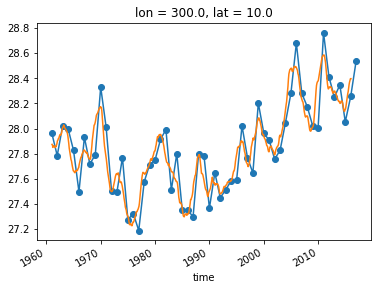
Let’s illustrate by selecting a single point.
[35]:
sst_ts = ds_all.sst.sel(lon=300, lat=10)
sst_ts_annual = sst_ts.resample(time='A').mean(dim='time')
sst_ts_annual
[35]:
- time: 57
- dask.array<chunksize=(1,), meta=np.ndarray>
Array Chunk Bytes 228 B 4 B Shape (57,) (1,) Count 456 Tasks 57 Chunks Type float32 numpy.ndarray - time(time)datetime64[ns]1960-12-31 ... 2016-12-31
array(['1960-12-31T00:00:00.000000000', '1961-12-31T00:00:00.000000000', '1962-12-31T00:00:00.000000000', '1963-12-31T00:00:00.000000000', '1964-12-31T00:00:00.000000000', '1965-12-31T00:00:00.000000000', '1966-12-31T00:00:00.000000000', '1967-12-31T00:00:00.000000000', '1968-12-31T00:00:00.000000000', '1969-12-31T00:00:00.000000000', '1970-12-31T00:00:00.000000000', '1971-12-31T00:00:00.000000000', '1972-12-31T00:00:00.000000000', '1973-12-31T00:00:00.000000000', '1974-12-31T00:00:00.000000000', '1975-12-31T00:00:00.000000000', '1976-12-31T00:00:00.000000000', '1977-12-31T00:00:00.000000000', '1978-12-31T00:00:00.000000000', '1979-12-31T00:00:00.000000000', '1980-12-31T00:00:00.000000000', '1981-12-31T00:00:00.000000000', '1982-12-31T00:00:00.000000000', '1983-12-31T00:00:00.000000000', '1984-12-31T00:00:00.000000000', '1985-12-31T00:00:00.000000000', '1986-12-31T00:00:00.000000000', '1987-12-31T00:00:00.000000000', '1988-12-31T00:00:00.000000000', '1989-12-31T00:00:00.000000000', '1990-12-31T00:00:00.000000000', '1991-12-31T00:00:00.000000000', '1992-12-31T00:00:00.000000000', '1993-12-31T00:00:00.000000000', '1994-12-31T00:00:00.000000000', '1995-12-31T00:00:00.000000000', '1996-12-31T00:00:00.000000000', '1997-12-31T00:00:00.000000000', '1998-12-31T00:00:00.000000000', '1999-12-31T00:00:00.000000000', '2000-12-31T00:00:00.000000000', '2001-12-31T00:00:00.000000000', '2002-12-31T00:00:00.000000000', '2003-12-31T00:00:00.000000000', '2004-12-31T00:00:00.000000000', '2005-12-31T00:00:00.000000000', '2006-12-31T00:00:00.000000000', '2007-12-31T00:00:00.000000000', '2008-12-31T00:00:00.000000000', '2009-12-31T00:00:00.000000000', '2010-12-31T00:00:00.000000000', '2011-12-31T00:00:00.000000000', '2012-12-31T00:00:00.000000000', '2013-12-31T00:00:00.000000000', '2014-12-31T00:00:00.000000000', '2015-12-31T00:00:00.000000000', '2016-12-31T00:00:00.000000000'], dtype='datetime64[ns]') - lon()float32300.0
- standard_name :
- longitude
- pointwidth :
- 2.0
- gridtype :
- 1
- units :
- degree_east
array(300., dtype=float32)
- lat()float3210.0
- standard_name :
- latitude
- pointwidth :
- 2.0
- gridtype :
- 0
- units :
- degree_north
array(10., dtype=float32)
[36]:
sst_ts.plot()
sst_ts_annual.plot()
[36]:
[<matplotlib.lines.Line2D at 0x7fc69021b210>]
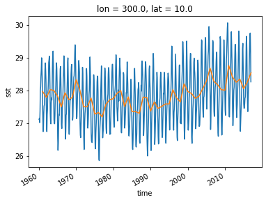
An alternative approach is a “running mean” over the time dimension. This can be accomplished with xarray’s .rolling operation.
[37]:
sst_ts_rolling = sst_ts.rolling(time=24, center=True).mean()
sst_ts_annual.plot(marker='o')
sst_ts_rolling.plot()
[37]:
[<matplotlib.lines.Line2D at 0x7fc690109d10>]
Finale: Calculate the ENSO Index
This page from NOAA explains how the El Niño Southern Oscillation index is calculated.
The Nino 3.4 region is defined as the region between +/- 5 deg. lat, 170 W - 120 W lon.
Warm or cold phases of the Oceanic Nino Index are defined by a five consecutive 3-month running mean of sea surface temperature (SST) anomalies in the Niño 3.4 region that is above (below) the threshold of +0.5°C (-0.5°C). This is known as the Oceanic Niño Index (ONI).
(Note that “anomaly” means that the seasonal cycle is removed.)
Try working on this on your own for 5 minutes.
[ ]:
Once you’re done, try comparing the ENSO Index you calculated with the NINO3.4 index published by NOAA. The pandas snippet below will load the official time series for comparison.
[38]:
import pandas as pd
noaa_nino34 = pd.read_csv('https://www.cpc.ncep.noaa.gov/data/indices/sstoi.indices',
                          sep=r" ", skipinitialspace=True,
                          parse_dates={'time': ['YR','MON']},
                          index_col='time')['NINO3.4']
noaa_nino34.head()
[38]:
time
1982-01-01    26.72
1982-02-01    26.70
1982-03-01    27.20
1982-04-01    28.02
1982-05-01    28.54
Name: NINO3.4, dtype: float64
Getting Help with Xarray
Here are some important resources for learning more about xarray and getting help.